CHAPTER III-MOON'S TOTAL CHARGE

MOON's TOTAL CHARGE ON E.M

Every previous solution is solved with many assumptions. Anyhow, the results are meaningful; they do confirm that the semi-moons in every day of Moon are approximately the reverting points when the Moon’s hemisphere effect changes from negative to positive or vice versa. Hence the two semi-moons divide the Moon’s orbit into 2 different, opposite halves; the effect on one half is going against or contrarian the current E.M, while the other’s effect is supporting or backing the current E.M.

The radiation from the Sun is changing and the Moon charge therefore is changing accordingly; so there must be a sequent change in Moon’s effect on E.M, and this chapter is a discussion about the change in circumstance when Moon’s charge is changing and the total charge ‘’Qa+Qb’’ is no more a ‘’0’’.

We leave the influence of permeability of the media between Moon and Earth centre for another problem; just consider the Moon’s influence on Earth’s surface.

Let’s set and solve the following problems for Moon’s effects.

2/-The problem of Moon’s total charge for Houston:

Houston of U.S chosen as observer in this problem is rather close to Earth's equator and quite in the middle of Van Allen belt and plasma sphere; therefore, it is very hard to detect the Moon’s effect. Nonetheless, we keep working with that location as observer then sort out the issue, and following is the problem:

U.S observer location (30N, 95W), USA on 02^nd May 2017, Moon’s total charge Qm and other parameters:

-Illumination: 49.1%≈50%, this is to make sure that each of the two hemispheres is capable to eliminate the other, so the hemispheric effect can be null.

-Meridian passing: 19.31 hrs.

-Moon rise/set (excerpt from Moon’s time table):

-Distance: 377652 km from point P to Moon.

-Moon’s average radius: R=1738.1 km.

Question:

With Moon’s total charge Qm≠0, consider the amplitude of magnetism that directly induced by Moon on Houston at 19.00 hrs LT.

2/1-To understand more about the question (analysis):

-The meridian passing is on 19.31 hrs at 75.7⁰.

-From the Moon’s timetable: Moon rise/set is 12.38/(next day)02.20 hrs. or 12.38/26.20  (or Moon’s on sky within 822 minutes).

-The distance from A or B to a general P (on longitude of P) can be viewed as the same and depicted in the following figure:

  

-The given P is on land surface with eye height ‘’0’’, the horizon viewed from P is a plane with the straight line from Sunrise (A) to Sunset (B).

-Note that AP = PB, by Pythagorean theory AP=(AO²-OP²)^1/2 (Figure 4/IV), where OP=Re, the value of Earth average radius despite ‘’O’’ is not coinciding on Oe (Figure 5/IV).

-A circle with centre (O) is designed to meet AP=(AO²-OP²)^1/2 and distance from P to Moon 377652 km. This centre (O) may not be coinciding on the terrestrial geometric centre (Oe).

 2/2-Solution:

2/2/1-Step 1: to re-think about the real things.

Like any other electric current or moving charge, the Moon definitely contributes magnetism. Moon’s total charge has been assumed as neutral with 2 opposite hemispheres in previous problem.

But in reality the total charge of any object under solar wind can’t be neutral at all the time; it is actually changing, and is given a value Qm (positive) in this problem.

The questions are how magnificent is the magnetism induced by the lunar total charge? Which wise (north or south) does it direct to?

2/2/2-Step 2: Assumptions.

- P (30N, 95W) is assumed as the stance for observer with eye height ‘’0’’.

- Distance from P to A is the same as P to B or any position on the longitude of P to those 2 positions of Moon.

-The Moon is assumed as on ‘’no real move’’ throughout the time of calculation. By this condition, the Moon’s real move is not considered. Instead, we consider the Moon’s relative move or 12(+) hr. trace around the Earth.

-Moon’s total charge (Qm=Qa+Qb and Qm≠0) stays unchanged throughout this calculation.

-Distance: 377652 km is from P to the nearest position of the Moon. The distance from P to charge centre of Moon can be approximately added with ½ of Moon’s average radius 1/2*1738.1 km.

The distance d=378521 km is assumed as distance from observer to Moon’s charge centre.

3-Step 3: Solution with reliable accuracy.

-Recall Biot-Savart expression for a single charge. We add some more lines on the basic figure 12b/v to facilitate the solution.

-In the above figure:  The relative Moon’s trace (not the Moons’ orbit) in 12 hrs is demonstrated (from Moonrise till Moon set) in 2D coordinates, the larger half of the circle (from A to B through under part) is not viewed. Within this duration, the Earth completes almost a half of cycle around its own axis. We can imagine that a certain observer standing somewhere near either North or South Pole, with a restricted view she/he can observes the Moon rising like depicted in the figure (while the Moon after Moonset is not seen, and the Earth makes no move).

The problem becomes pure geometric on 2D coordinates; and the figure requires some additional assumptions and quantities:

+Moon is at a general position (M) on sky, its distance to P is ‘’r’’ which varies against time and reaches the given value of d at meridian passing;

+Moon is rising at A and setting at B;

+Moon is expecting to pass meridian at Z over P; where angle APM=angle APZ =90⁰ while Moon’s altitude reaches its max of that day 75.7⁰.

+Vector  ''v'' is perpendicular to the radius that drawn through Moon (OM);

+PD is perpendicular to OM and parallel to;

+The angles are named after each point and numbered: M1, M2 and O1,O2; or P1,P2,P3,P4;

+Parameters: d=378521*10³m (minimum distance from the given position P to Moon’s centre).

+The Moon’s angle (P2 or angle APM) is taken by a professional equipment (Sextant) (at the given time); (the ‘’altitude’’ of Moon or any object on sky is understood as the angle between the line from observer to the object and horizontal plane at observer. Therefore, a large gap between the two aforementioned concepts (altitude and P2) is found, and no chance for a mixing up or confusion). Nonetheless, we can’t deny that the Moon’s altitude depends on P2 and reaches max almost at the middle of Moon’s trace between A and B, therefore we may keep considering altitude in relation with Moon’s angle P2. Furthermore, by the laws of 3D trigonometric, we can calculate P2 from altitude or vice versa, but no discussion for that issue is encouraged in this book.

The following is a figure that depicts approximately the altitude of Moon and the Moon’s angle P2:

 Figure 9/V-Moon’s altitude

(At Moon’s meridian passing, the angle APM is obviously 90⁰ or ½ π while Moon’s altitude keeps varying (angle MPH is not always to be 90⁰ even if we measure it from Earth equator)).

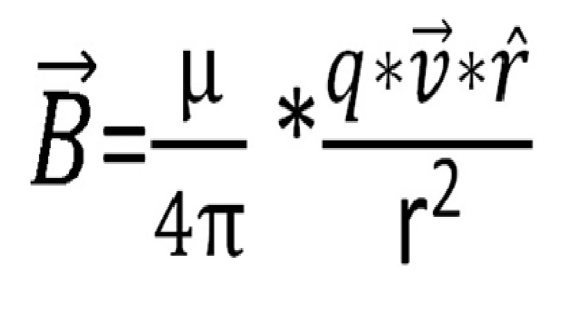
Again, we refer to the basic expression of Biot-Savart:

With Biot-Savart expression, this problem is the normal geometric one in astrophysics, we can demonstrate every important parameter on 2D coordinates. The sensitive issue in this expression is the product of vector ''v''  and unit vector ''r'', a vector directs from this page toward reader, and its  non-directional value is:

v*Sin(M1)

The non-directional value of B is:

b/1- To seek for (r ):

+Consider the triangle MDP (Vector ''v'' and PD are extended for a better view with M’P’//MP):

 Cos(O2)=Cos(07.95⁰)=0.990389

+In the triangle MPO:

In the triangle ODP:

OD=Re*Cos(O2)= 6356.8*0.990389=6295.704795 km

And Sin (M1) = Sin(81.91⁰+07.95⁰)=0.99999

MD = MO-OD or MD=(Re+d)-Re*Cos(O2)=6356.8+378521-6356.8*0.990389=

=378582.0952048 Km

Thus, r=MD/Sin(M1)= 378582.0952048/0.99999 =378585.88106 km=

r=378585.88106*10³m.

b/2-Angle M1:

M1=P2+P3 (Vector v is parallel with PD, the rule for alternate angles is applied)

P2 is Sextant reading (or astronomy almanac), and the P3=O2. Thus:

Angle M1=P2+O2, with given P2=81.91⁰ and P3=07.95⁰   

 Angle M1=81.91⁰+07.95⁰=89.86⁰ = 89051’’

Final calculation:

-Replace the followings in the expression and calculate value of B(tc):

Radius r=378585.881*10³m

Speed v=21230.8834 m/s

Angle M1=89⁰51”, Sin(M1)=0.99997≈1.

As assumption of this problem, q=Qm Coulomb, every length is in meter (m), the unit of B is Tesla (T).

We have:

B(tc)=10^-7*21230.8834*378585.881^-2*10^-6*Qm=

=1.481287*10^-20*Qm Tesla

(The previous approximate calculation gives result: B(tc)=1.439480*10^-20*Qm)

Because every of (r,v,M1) is depending on observer’s position, therefore the above result cannot be used for everywhere. Nonetheless it is to confirm that the Moon exerts its static electric force on the

Earth and especially induces a magnetic field on it, the value can be calculated.

For instant, a reading on a Tesla meter is indicating that the Moon’s contribution at Houston (South U.S.A) reaches its max +5*10^-7 T (normally the meter reading about 2-3 hrs before meridian passing can indicate the average magnetic level); we can find Moon’s total charge as following:

B(tc)= 1.481287*10^-20*Qm=5*10^-7 Tesla

Qm=B(tc)/ 1.481287*10^-20=5*10^-7/ 1.481287*10^-20 =

=3.375443*10¹³ Coulombs.

Everywhere inside the loop, the magnetic vector is by right-hand law.

(Problem: (the following problem is designated for 60 N to make sure that Moon signal is detected without being totally barred by plasma sphere): 3.375443*10¹³ Coulombs is a value of Moon’s charge that we detected when semi-moon (illumination 50%) is passing meridian of a position ‘’P’’ (60N, 0.0). If in 36 hrs later, when Moon’s illumination of 40% we detect Moon’s charge to be ‘’0’’ at a certain position P’ (60N, 180.0). Calculate the Moon’s total charge components Qa & Qb? 

This theoretic problem is definitely inspired by many science students but not included in this book. After this problem, we find out more about the roles of 2 hemispheres of Moon on E.M).

Figure 13/V-Earth’s magnetic field amplitude (in mG)

The above is a real graph of magnetic amplitude observed by our correspondent at latitude 70 N on Atlantic, about new moon. The records are bold for 10 minutes before and after the Moon’s meridian passing.

CHAPTER I/p2-VAN ALLEN BELT CONTRIBUTION

VAN ALLEN BELT

I-General about Van Allen belts:

I and many among my colleagues used to view Earth’s magnetic field as one that can only facilitate the magnetic compass to indicate the North magnetic direction and no more it can offer. But the Van Allen belt appears to change our mind; the Earth’s magnetic field is not very strong but good enough in facilitating the establishment of Van Allen belt which can stop any fast moving charged particle. The Van Allen belt, as matter of fact, plays an important role in protecting our planet.

(The following is almost prepared with close reference to SPACE & NASA’s documents and papers, which are open to everyone and nothing is from classified information.)

(By NASA)

1-What is Van Allen belt: a collection of charged particles, gathered by Earth’s magnetism, in a shape of belts around Earth.

2-The earliest discovery to the belts: 1958 by Explorer 1 (NASA’s Satellite).

-Belt’s structure: normally 2 belts, one is separated from the other by a large drain/gap; can split up to 3 belts or merged in one sometimes. The inner belt is almost close to Earth surface at minimum about 400 miles; while the outer belt is rather far and even stretches to 36000 miles.

The drain is discovered in 2012; a remarkable feature of the belt is that its drain can stop the ultra-fast electron in there. The scientists from NASA are still not determined about reason for the belt separation. Their hesitation is quite understandable because no mechanism of electric force or magnetic field is found linking to the wax & wane activity of the belts (which is in conjunction with Sun’s activity). The scientists likely ascribe to the particles from space or the Sun.

The unidentified particles or quarks might be gathered among the belts and create an unknown field between them, the field makes the belts split-up wide.

-How the belts work: They can wax and wane in response to incoming energy from the Sun, sometime swelling up enough to expose satellites in low-Earth orbit to damaging radiation.

-Undiscovered about the belts: With some satellites working on space at all the time; the more research to the belts are carried out, the more expect to be discovered; even the unidentified particle or quark.

-Plasmasphere: A companion to the belts is a giant plasma sphere which can be assumed as twinned to the belts. The plasma sphere is cloud of relative cool and charged particles that fills the outermost region of Earth’s atmosphere. That sphere begins approximately at 400-600 miles (rather close to Earth surface) and extends partially to outer Van Allen belt.

PROBLEM

If total charge of the Van Allen belts and plasma sphere is equivalent to a single band of +10⁶ Coulombs around Earth equator at a distance 1500 km from Earth surface, and evenly distributed on it.

How is the magnetism induced by the Band to the equator (Earth)? 

(V-A 01)

   

    

Where unit of ‘’Q’’ is in Coulomb and unit of ‘’d’’ is km.

Replace Q=10⁶ Coulombs, d=1500 km (as assumed) into the above formula:

  Δ(3)= -8.4169*10^-23 *666.666667=10^-20*5.611267 Tesla

(Note: the Belt is assumed as on a plane perpendicular to Earth’s rotating axis, the assumption is not verified and the reality definitely is not be so. Therefore, in order to calculate for a better accuracy, the belt as well as the plasma sphere can be represented by many bands (or hoops) in a larger problem).

Conclusion:

If Van Allen belt and plasma sphere are equivalent to a band of Q Coulombs (the Band) around the Earth on plane of Earth’s equator. The Band is to induce magnetism on Earth’s equator; its additional intensity is calculated as (V-A 01):

 

In reality, Van Allen belts and plasma sphere are not only changing in shape and size, but also in intensity. With such a complicated change, the above mentioned ‘’Δ3’’ demonstrates nothing but ‘’yes’’ to the question ‘’influence?’’. Furthermore, as noted above, the larger problem is required to estimate the additional magnetic intensity with better accuracy.

PREAMBLE

PREAMBLE

Earth Magnetism or E.M is one of the oldest themes in the Earth study. The world scientists are researching, debating about the same theme for several decades; I assume that there is not only one but some of them even dropped it.

I am neither going to deny the settled theories about E.M nor to make the Geomagnetism up-side-down, but consider the E.M as one constituted by 2 major parts. The ‘’part I’’ mainly presents the contributions from the charges at sea surface and land surface. The other one is a massive part that contributed by external magnetic inducers such as Van Allen belt, Moon and atmosphere; a shocking extra chapter is the magnetism at The Poles.

The mechanism in magnetic inducement of E.M is rather complicated and likely to be ruled by some principles that had not been mentioned so far; each spot on the Earth is different to any other.

The very special paradox is that ‘’land charges versus sea surface charge in contributing to the E.M whilst they both are moving together with Earth’s rotation’’. Although land charges and sea surface charge are influenced by external movement, I do keep them in a separate part (Part I) for a better discussion.

Actually I leave what happen inside the Earth as the stuff of a conservatory; just add something on the settled basis with some effects on Earth surface and from sky.

Many scientists assume that the astronomic objects may contribute several per cents in the E.M. In this book, I argue that the contribution from those might go beyond any previous prediction and certainly it must not be such tiny as assumed by those scientists…

E.M is a giant theme like the huge size of the Earth. I am capable and proud to interpret some of the information that compiled by many scientists in history and especially in about a century time.

Furthermore, like any other semi-empirical study, this book presents some latest E.M data and I analyse them with my own view. On some aspect, this book is more likely presenting a discussion by which I contribute my own view to a theme that researched by tens of scientists in the world.

Like any other book, this is compiled with reference to many books as well as researching reports from many scientists in the world. The knowledge from electricity to atmosphere, from math to physics; all of them are referred to facilitate the research.

The Earth rotation is definitely to suggest us that E.M is created by the rotation, or the Earth is viewed as an electromagnet. I trust that the E.M must look alike a normal magnet if we eliminate all external compositions (but I don't attribute the astronomic power as reason for the gap between North magnetic pole and the geometric one).

The above assumption has been the subject of much and long study, particularly by S.J. Barnett, who has shown that a piece of iron may be magnetized by rotation.

In 1900, Sutherland suggested a possible cause of the Earth Magnetism the rotation of an electrostatic field within the Earth –a positively charged core and a negatively charged crust, or vice versa.

The later analysis made by Bauer in 1922, using improved data based on modern observations, gave approximately the same result.

Sutherlands, Bauer and Swann suggested that we may have to look for some slight but fundamental modification to those accepted laws.

(Magnetic storm) it was recognized that the more severe magnetic disturbances occur at practically the same time all over the Earth, and further comparative study of abrupt beginnings and sharp turning points indicated strict simultaneity.

The world scientists keep researching the Earth as well as E.M at all time. The followings are some information in brief about the science achievements:

-Temperature at Earth’s inner core boundary: by measuring the melting point of iron at high pressure (about 2.2 million times more than normal pressure on Earth surface) in laboratory, the scientists drew a result to calculate the temperature now estimated at 6,000 ⁰C (about 10,800 F), that’s as hot as the surface of the Sun?

-Earth’s inner core is solid, while its outer core is molten or loose then crust and mantle above the outer core. Along with Earth’s spin they create the magnetic field?

X

X                                             X

Before any further discussion about E.M, we should not neglect the following from an important book ''TERRESTRIAL MAGNETISM''.

Quote:

In the previous centuries, the XIX and XX, human being had carried out a series of attacks to the Earth Magnetism, the questions are: What it is, What caused it, What cause it to change. Many leading physiscists, mathemeticians joined in those attacks. Many theories, one after another had been advanced then withdrawn if it was found inconsistent with some of the observed facts.

1/They are inadequate or inconsistent because:

-Can fit well with quality but can’t do with quantity.

-Can fit well with primary stage but can’t do with the next when our knowledge is improved.

2/The advances in other field of science have been employed:

-Cathod rays, electronic theory of matter.

-Constitution of the Sun.

-Earth interior.

3/Gilbert’s conception: Earth is a great magnet uniformly magnetized about the Earth own rotating axis. This theory is discarded afterward when the high temparature inside the Earth is recognized by then some material is demagnetized in such high temparature condition.

4/Under high pressure: properties of some matter in great pressure may be materially different from those observed in normal condition. Susceptibility to magnetization is one of those properties. Some geophysicists suggest that the Earth’s inner core is composed by almost entirely Nikel and Iron and a possibility of susciptibility of magnetization in spite of high temparature, because of enormouse high pressure. Some magneticians are inclined to work further to consider The Earth as a giant magnet.

5/ Electric currents flowing around The Earth: When it seemed clear that the conception of the Earth as a permanent magnet could be sustained, the idea was advanced that the Earth magnetic field might be due to electric currents flowing about the Earth, either below the surface or in the atmosphere-the Earth an electromagnet.

6/Three portions constituting the E-magnetism: The mathematical analysis of the Earth magnetic field, according to the method devised by Gauss and extended by Neumayer and Peterson (1891) and Schmidt (1896), indicated that:

-A portion of Earth Magnetism, perhaps one-fortieth, could be referred to forces outside the Earth.

-Another small portion to vertical electric currents.

-But by far the larger part to a system of force within the Earth.

A new analysis made by Bauer in 1922, using improved data based on modern observations, gave approximately the same result. He reached the conclusion that for a satisfaction representation of the observed data it is necessary to recognize the existence of an internal magnetic system constituting about 94 per cent of total field, with an external system and a non-potential system each amounting to about 3 per cents.

A comparison of his results with those previously obtained for the epochs: 1842 and 1885 indicated that the intensity of magnetization of the Earth had been decreasing during the 80 years at an average annual rate of one part in 1,500; a rate of loss which it is hard to reconcile with the age of Earth and the present intensity of magnetization unless we suppose that there have been also periods of increasing intensity.

7/ E-Magnetism caused by Earth’s rotation: The idea of Earth as an electro magnet naturally suggested the possibility that its magnetism may be caused by its rotation. This possibility has been the subject of much study, particularly by S.J. Barnett, who has shown that a piece of iron may be magnetized by rotation, though the observed effect was much too small to account for Earth Magnetism.  In 1900, Sutherland suggested as a possible cause of the Earth Magnetism the rotation of an electrostatic field within the Earth –a positively charged core and a negatively charged crust, or vice versa.

8/ Electronic theory and Sutherland: The development of electronic theory of matter, with the atom consisting of a positively charged nucleus surrounded by negatively charged electrons, led Sutherland to suggest that if for some unknown reason, connected perhaps with gravitation, the negative charge of the atom is farther from centre of Earth than the positive charge by only 4x10^-9 cm, it would account for a magnetic field comparable with that of the Earth. When the electronic theory had been more fully developed and Sutherland’s hypothesis submitted to further test, it was found to be untenable either qualitatively or quantitatively.

Failing to find a satisfactory explanation to the Earth’s magnetism on basis of the known properties of matters and accepted laws of electrodynamics, Sutherlands, Bauer and Swann suggested that we may have to look for some slight but fundamental modification of those accepted laws, possibly as regard the mutual attraction and repulsion of moving positive and negative electrons, similar to a suggestion of Lorenz regarding the cause of gravitation. Indeed there seems to be growing a belief that gravitation and terrestrial magnetism are very closely allied and probably to be traced to a common origin.

9/ Atmosphere electric & Earth currents: In view of difficulties in the way of a direct solution of the problem of the cause of Earth Magnetism, the magnetism researchers have turned their attention to a study of its variations and their correlation with associated phenomena, such as atmospheric electricity, Earth currents, aurora, sun spots, solar radiation, in the hope that the cause of variations may be discovered, and that in that way light would be thrown on the main problem. In particular, magnetic storms, those irregular disturbances of large amplitude and comparatively short duration, have been the subject of much study.

It frequently happens that the occurrence of magnetic storms and auroras coincides with the presence of large spots on the sun, and this naturally has led to attempts to trace a causal relationship. It was soon seen that a direct magnetic effect by the sun was out of the question, because of great distance. With the development of the idea that the Earth’s magnetism may be caused by current of electricity, different forms of electric discharge emanating from the sun were successively put forth as the cause of observed terrestrial phenomena, the theories advanced keep pace with the development of our knowledge of electrical discharges in vacuum.

The correlation between magnetic storms with sunspots, although very satisfactory when based on yearly average, leaves much to be desired when individual cases are considered. Thus severe magnetic storms sometimes occur when no large sunspots are visible, and on the other hand a sunspot is not always accompanied by a magnetic storm. Large magnetic storms always follow each other at an interval approximating the time of revolution of the sun and such reoccurrence has been traced with several rotation periods, not every recurrence is accompanied by a sunspot, however.

10/ Maunder hypothesis:

 To meet these conditions, Maunder advanced the hypothesis:

-The solar activity which gives rise to magnetic disturbances on the Earth does not act equally in all directions but along narrow well-defined streams, not necessarily truly radial.

-These streams arise from active areas of limit extent.

-These active areas are not only the source of our magnetic disturbances but are also the seats of formation of sun spots.

-These areas can be active both before a spot has formed and after it has disappeared.

Birkeland, Arrhenius, and Normannd agree to consider aurora as a luminescence produced by the absorption of cathode rays in the upper atmosphere and attracted toward the Earth magnetic poles. Birkeland, who devoted many years to the study of auroras, advances a theory that cathode rays from sun can set up electric currents in the atmosphere which in turn give rise to secondary cathode rays. He supported his theory by the production of artificial auroras in laboratory, about a magnetized steel ball in a tube of rarefied air exposed to cathode rays.

11/ Sun’s electrified particle streams:

If magnetic disturbances on the Earth are to be ascribed to streams of electrified particles shot out from the sun, we should expect to find a disturbance occurring first at the part of the Earth first entering the stream and later at other places as they in turn entered the stream, as a result of the combined motion of the Earth in its orbit and the sun about its axis. From the time of the earliest comparison of photographic records from widely separate observatories, it was recognized that the more severe magnetic disturbances occur at practically the same time all over the Earth, and further comparative study of abrupt beginnings and sharp turning points indicated strict simultaneity, the departures therefrom being ascribed to errors inherent in the time measurements, so that the more accurate determination of the time of occurrence of such salient features was suggested as a method of determining differences of longitude.’’

Unquote

The latest document for the same theme-the Earth’s magnetic field, is one from a French Scientist; I would like to cite here a short excerpt from his argument:

Quote

THE ORIGIN OF THE EARTH’S MAGNETIC FIELD: FUNDAMENTAL OF ENVIRONMENTAL RESEARCH? (Emmanuel Dormy-MHD in Astro-and Geophysics, Department De Physique, LRA, Ecole Normale Superieure-France.)

The origin of The Earth’s magnetic Field is a long-standing issue, which has captured attention of many reknown scientists. If William Gilbert, Andre-Marie Ampere, Rene Descartes, Edmond Harlley, Kart Friedrich Gauss, Lord Brackett and many others who contributed to the development of science, have worked on this problem, it is mainly because it related to a very important issue of very critical importance: navigation at sea. This is not so true any more, now that satellites provide the precise latitude and longitude without the need for us to rely on Earth’s internal magnetism. Yet the question of origin of Earth’s magnetism is so natural that it is still an object of very competitive research. Nobody can ignore that the compass needle points toward the North, and it is a bit irritating that we still can’t not offer a complete physical understanding of why it is so. The problem therefore becomes an active field of fundamental research in which significant progress has been made in the last few years using combined theoretical, experimental and a numerical approach. By its very nature, the problem is interdisciplinary and lies at the interface of physics, geophysics and applied mathematics. This problem has recently received considerable attention in the press because of concern of a possible reversal of polarity of the Earth’s magnetic field in the near future. Considering that we risk seeing our planet unshielded from solar wind, understanding the field generation mechanism again appears to be a societal concern and a legitimate goal of environmental research.

’THE ORIGIN OF EARTH’S MAGNETIC FIELD

When the Earth formed in 4.5 billion years ago, heavy elements concentrated at centre, as result 3000 km below our feet lies the largest of our planet’s oceans: the core of liquid iron (mixed with traces of light elements), a sphere of 3400 km in radius. As the pressure increases towards to the heart of the Earth, the iron solidifies and we find a solid inner core, which occupies a volume of 1200 km of radius. It is the metallic core that the magnetic field of the Earth originates. Temperatures at such depth are above 3000 degrees K and thus well above Curies point (at which metal loses its ferromagnetic properties). A magnetic field can therefore only be sustained if electrical currents circulate in this ocean of liquid iron. However, Ohmic dissipation would suppress any unsustained electrical current in the Earth’s core...’’

Unquote

About the same theme, we can’t ignore the following that cited from an academic literature of science in United Kingdom. At the first page we find right away:

Quote

unquote 

We have gone through many theories but not the following combined theory which is most read at present time:

‘’The Earth and most of the planets in the Solar System, as well as the Sun and other stars, all generate magnetic fields through the motion of highly conductive  fluids. The Earth's field originates in its core. This is a region of iron alloys extending to about 3400 km (the radius of the Earth is 6370 km). It is divided into a solid inner core, with a radius of 1220 km, and a liquid outer core. The motion of the liquid in the outer core is driven by heat flow from the inner core, which is about 6,000 K (5,730 °C; 10,340 °F), to the core-mantle boundary, which is about 3,800 K (3,530 °C; 6,380 °F). The pattern of flow is organized by the rotation of the Earth and the presence of the solid inner core. 

The mechanism by which the Earth generates a magnetic field is known as a dynamo. A magnetic field is generated by a feedback loop: current loops generate magnetic fields (Ampère's circuital law); a changing magnetic field generates an electric field (Faraday's law); and the electric and magnetic fields exert a force on the charges that are flowing in currents (the Lorentz force). These effects can be combined in a partial differential equation for the magnetic field called the magnetic induction equation:

...where u is the velocity of the fluid; B is the magnetic B-field; and η=1/σμ is the magnetic diffusivity, a product of the electrical conductivity σ and the permeability μ. The term ∂B/∂t is the time derivative of the field; ∇  ² is the Laplace operator and ∇   is the curl operator.

The first term on the right hand side of the induction equation is a diffusion term. In a stationary fluid, the magnetic field declines and any concentrations of field spread out. If the Earth's dynamo shut off, the dipole part would disappear in a few tens of thousands of years.

In a perfect conductor (σ=∞), there would be no diffusion. By Lenz's law, any change in the magnetic field would be immediately opposed by currents, so the flux through a given volume of fluid could not change. As the fluid moved, the magnetic field would go with it. The theorem describing this effect is called the frozen-in-field theorem. Even in a fluid with a finite conductivity, new field is generated by stretching field lines as the fluid moves in ways that deform it. This process could go on generating new field indefinitely, were it not that as the magnetic field increases in strength, it resists fluid motion…’’

Although I am writing purely about external influence, I must make an unforgivable mistake if I don’t mention these issues:

-The gap between Earth’s rotation axis and magnetic pole: This issue will be re-compromised in the conclusion of this book. However, one of hypothesises about the origin of Earth Magnetism presumes that the ‘’yolk’’ of the Earth, which induces the Earth Magnetism, used to be together with Earth’s rotation axis but shocked by a huge meteorite then turns North side South. The ‘’turn’’ has not been perfect and leaves the North Magnetic pole far from geometric North pole (about 11⁰-17⁰). By that author, the collision with the huge meteorite made a very serious disaster to the living in Dinosause Era, when all the Dinosause dead.

-The deviation and magnetic-longitude of ‘’0’’ deviation.(Magnetic susceptibility of material).

The relevant documents may build a huge pile; we can’t read every one of them but the following magazine- The GEOMAGNETISM-Magnetic Model and Navigation. The paper is to affirm that ‘’the study of geomagnetism is one of oldest geophysical sciences. Geomagnetic fields have been observed and been used from ancient time.’’ That paper also emphasizes that the magnetic compass needle does not point toward the North Magnetic Pole, but in the direction of the magnetic field line-horizontal composition-at the place where the compass is located.

On the scope of International cooperation in research, the paper introduces World Magnetic Model (WMM), a joint product of the United States National Geospatial Intelligence Agency and United Kingdom Defence Geographic Centre. This model is used by many giant and important bodies such as U.S Department of Defence, NOAA, U.K ministry of defence, NATO, International Hydrographic Organization (IHO).

The paper is interesting and to be one of viable information sources for the author of this book.

The latest information from a science magazine is the model of some French scientists.

 Image 7/F-Earth Magnetism produced in the core

''The Earth core is supposed to be filled with molten Magnesium since Earth’s violent birth. The flow or move of the molten in Earth core is to produce Earth Magnetism.''?

Anyhow, those scientists must satisfy themselves as how the magnesium can be mixed together with iron, even if the molten magnesium is found in there.

PART I

Some viable concepts and

The Sea vs Land contributions to Earth Magnetism

Chapter I

VIABLE RELEVANT CONCEPTS

Nowadays, the quantum theory is the first and the most that catch the attention of the people in the world. Nonetheless, we should recognize that the physics can’t be just bracketed in quantum, and so we got to look backward some centuries when we can find W. Coulomb, A.Ampere and the two others J.B.Biot and F.Savart. 

I-Static Electric Charge and Coulomb:

This is the first we inspire when discuss about Earth Magnetism, the subject is attached to a scientist who discovered electric charge: W. Coulomb.

His rule is simply expressed in a formula for the force (F) between the two charges:

F=k_e*q₁*q₂/r²

Or

=k_e*q₁*q₂*r^-2

Where q1 and q2 are values of charges, each can be either (-) negative or (+) positive. The distance between the two is ‘’r’’ and the Coulomb constant ‘’k_e’’ is depending on the media between the two.

 ke=8.99*10⁹ N.m².C^-2: Coulomb constant for the normal environment or vacuum between the two charges. The force is found to be negative (-) when either q1 or q2 is negative; to be positive (+) when both of them are positive or negative; this is quite a law in math and it demonstrates the wise of force ‘’+ push’’ or ‘’- pull’’.

Portrait of Charles-Augustin de Coulomb

Charles-Augustin de Coulomb was an eminent French physicist. He formulated the Coulomb’s law, which deals with electrostatic interaction between electrically charged particles. The coulomb, SI unit of electric charge, was named after him.

We are considering ‘’ke’’ for the media of large scale and complicated, therefore we should give out some assumptions before any problem.

Some more about moon-earth relation and calculation are debated in the ‘’Moon charge and E.M’’ of this book.

II-A. Ampere:

The second scientist we inspire is A. Ampere, he is a great scientist but simply his rule should be taken as: total charge in Coulomb transported through a point within a unit of time (second) is to make current value one Ampere.

(Portrait of André-Marie Ampère)

André-Marie Ampère (1775-1836) is a French Physicist and Mathematician; He worked at the beginning of the 1800s in Paris, France. He used his mathematical and statistical skills to observe and measure natural occurrences that had been discovered by other European scientists. He went on to produce complete proof of the relationship between electricity and magnetism. He also developed a new way of classifying chemical elements. Amp (Ampere) or his name is given to basic unit of electricity.

With the above concept of electric current, an instant of the 5 different charges moving through a point in 5 seconds can make an average current in that interim as following:

2 Coulombs in 1^st second;

3 Coulombs in 2^nd second;

1 Coulomb in 3^rd second;

2 Coulombs in 4^th second;

4 Coulombs in 5^th second, can make a current of:

I = (2+3+1+2+4)/5=12/5=2.4 A

Figure 1/I-Electric current & magnetism around

As soon as an electric current is created, a magnetic field is established around it.

III-Biot-Sawart laws:

In physics, the momentum as well as the ‘’particle spin’’ is considered as the most interesting subject. Let’s leave the modern physics and work with these two scientists.

Jean Baptiste Biot – a French scientist (1774-1862)

Felix Savart-a French physicist (1791 -1841)

Those two French physicians are known as inventers to the law that named after the both, the Biot-Savart about electromagnetism.

1-Biot - Savart law: The kernel of the law is to say that a charge motion is to make magnetic field. A point ‘’P’’, at a distance ‘’r’’ from a conducting wire where the charge moves in, is in a magnetic field which can be calculated as following:

   

Where dB is additional magnetic field contribution induced by the current ‘’I’’, which is created by the directional move of a charge ‘’q’’. 

Figure 2/I-A charge move and its magnetism contribution to point P.

And ‘’ds’’ is a small segment of wire, both ‘’ds’’ and ‘’ȓ’’ are respective vector units of wire length and distance from the wire to ‘’P’’; and product of those is dB -an outward vector or the vector that comes toward reader as following figure.

µ₀ – permeability coefficient of environment, is 4π * 10^-7 in normal air or vacuum.

2-Biot-Savart problem of many moving charged points:

Our discussion is not the first but is the most interesting application of Biot-Savart law, which will be applied to almost every issue in this book. Instead of momentum and spinning, we work with charge and orbiting. The following is an excerpt from a manual on web.mit.edu.com (Mit. University web).

Quote:

The magnetic field due to 30 charges moving in a circle at a given observation point. The position of the observation point can be varied to see how the magnetic field of individual charges adds up to give the total field.

In the above figure (9.1.11), we show an interactive Shock Wave display that is similar to that in figure 9.1.10, but now we can interact with the display to move the position of observer about in space. To get a feel for total magnetic field, we also show a ‘’iron filings’’ representation of the magnetic field due to these charges. We can move the observation point about in space to see how the total field at various points arises from the individual contributions of the magnetic field of to each moving charge.

Note, however, that since a point charge does not constitute a steady current, the above equation strictly speaking only holds in the non-relativistic limit where v<<C, the speed of light, so that the effect of ‘’retardation’’ can be ignored.

The result may be readily extended to a collection of N point charges, each moving with a different velocity. Let the i^th charge qi be located at (x,y,z) and moving with velocity v, using the superposition principle, the magnetic field at P can be obtained as:

Unquote.

IV-Major historic notes:

This book is not written about industrial magnetism but the subject is vital to the contemporary life, therefore the following note must benefit the readers in general. On the other hand, some reader can’t get through this book without reference back these notes.

The above figure illustrates how a direct current induces the magnetism during flows through a coil.

1-Magnetic field intensity: This is defined as the ratio between the max magnetic flux density of a circuit to the permeability of free space.

H=B₀/µ₀

The magnetic intensity depends on the geometry of the circuit and the conduction current, not on the medium.

The total magnetic field in a magnetic material is due to the conduction current in the external circuit and the microscopic current developed in the material.

B=B₀+ µ_0*M

2-Field strength (H):

Definition: It is the force experienced by a unit north pole at a point in a magnetic field

H=F/m

Where F is the force, m is pole strength.

-If the field lines are more, then H is high and vice versa.

-Thus, the closer to the pole, the higher strength of field. 

Nowadays, magnet is applied in almost every equipment or even toy. The power of U-shaped magnet is known to everyone who is experienced with machinery work.

3-Magnetization:

a-Magnetic domains in an un-magnetised bar point to random directions.

b-A bar magnet is brought near the un-magnetised bar.

c-The magnetic domains point in the same direction, producing magnetism. N or S poles of adjacent domains cancel each other out.

d-The atomic magnets at both ends are free. This produces N and S poles at the ends.

e-The atomic magnets at the ends tend to fan out due to repulsion between the like poles.

The magnet and its force applied in industry are not magic; they are available in every material and everything, their force is null because every elementary magnet in there points to different directions or even one eliminates the other. The external magnetic force helps a certain bar in its adjacent area to re-direct every elementary direction and make a force of their total.  

4-Magnetic Equivalent Circuit:

Magnetic Field Intensity (H): the amount of field force (mmf) distributed over the length of the electromagnet. Sometimes referred to as Magnetizing Force.

Magnetic Flux Density (B)-The amount of magnetic field flux concentrated in a given area.

Where N-numbers of turns of coil; i-current in the coil; H-magnetic field intensity; l-mean length of the core.

Relation between B and H:

The magnetic field intensity, H produces a magnetic flux density, B everywhere it exists.

B=µH (weber/m²) or Tesla

B=(µ_r/µ₀)H(w/m²) or T

µ: Permeability of the medium.

µ₀: Permeability of free space=4π.10^-7 wbA.t.m 

µ_r=µ/µ₀ relative permeability of medium.

Magnetic Flux Φ

-Unit for flux is ‘’weber’’

-The definition of 1 weber is the amount of flux that can produce and induced voltage of 1 volt on a one-turn coil if the flux reduced to zero with uniform rate.

This concept is also defined as following: It is a measure of magnetic field in a certain medium. In simple term if the magnetic field has to pass through a certain medium, it will always travel as ‘’flux’’ lines (flux lines are imaginary, but continuous lines travelling from North pole to South pole of a magnet. Its units are Weber.

Magnetic Flux Density B

-Unit for magnetic flux density is Tesla.

-The definition of 1 tesla is the flux density that can produce a force of 1 Newton per meter acting a conductor carrying 1 ampere of current.

Magnetic Field Strength H

-Unit for magnetic field strength is Ampere/meter.

-A line of force that produce the flux.

Earth’s Magnetic intensity in history and now (an excerpt):

The above note is cited as some information about the Earth’s magnetism in history and now. Definitely Humphreys does not fabricate the graph, and he draws it with facts that found in researching. The question is ‘’steady decay’’ now and then?

V-Major Features & compositions:

1-E.M polarity: at present, south magnetic pole is nearly coinciding with earth north geographic pole, that’s why magnetic compass north hand always points toward North.

 

Figure-3/I-Earth Magnet with zero-deviation. 

The above image is set with assumption that magnetic deviation is ‘’nil’’, and South magnetic pole is on North geographic pole.

2-Earth Magnetic field in different coordinates:

The following is an excerpt from manual of Bremen University:

3-Earth Magnetic field compositions:

Earth Magnetism or E.M is contributed by several magnetic inducers, we are going to discuss about someone and not the whole. Unlike traditional way, our way is to start from inducers such as charge on continent, sea surface charge and Moon charge. Therefore we got to denote each magnetic composition with a number attached to a symbol ‘’Δ’’ such as Δ(1) or Δ(2), except B(e) which is induced by inner rotor of the Earth as well as local man-made source. B(e) is also denoted as Δ(7), the only one composition which has undefined direction and left as non-directional quantity, while all the rest are directional.

-Positive charge on land contribution: Δ(1), note that positive as well as negative charge is everywhere, but we do not consider every one as it is but with massive quantity as representative of each. Therefore a continent is positively charged in general. Direction of Δ(1) will be defined in its problem, the land charge contribution in chapter II of part I-‘’sea surface charge versus land charges’’.   

-Negative sea surface contribution: Δ(2), unlike continental surface which is positive, the sea surface is homogenous as only one electrode and always negative. The direction of this composition is defined in its problem, chapter II of part I.

-Van Allen belt contribution: Δ(3), Van Allen belt and its companion, the plasma sphere, are not just making a shield to protect the Earth, they are charged and to contribute to E.M. The direction of their contribution is defined in the problem in chapter I of part II.

-Negative moon’s hemisphere contribution: Δ(4), the Moon primarily is assumed as neutral with 2 hemispheres of 2 opposite charges. Each hemisphere is inducing magnetism to Earth different to the other. The direction of this quantity is defined in its problem in part II.

-Positive Moon’s hemisphere contribution: Δ(5), the shined hemisphere of Moon is positive as losing electrons under solar wind. It induces magnetism to Earth and its direction is defined in its problem in part II.

-Contribution of total charge of Moon: Δ(6), the above mentioned problems are considering Moon as neutral of 2 opposite charges, but in reality the total of those charges Q(a)+Q(b) rarely is neutral, besides a certain value different to Zero; therefore its contribution is considered and it has potential to be a huge surprise.

V-Two important characteristics of material:

These are not just 2 important characteristic of material, they are 2 subjects that attracts a lot of researchers in history and now. Although we can go along with the researchers but we can’t keep going ahead without some brief about them.

1-Permeability: The magnetic permeability of a material is the degree of magnetization that it receives when it responds linearly to a magnetic field. The symbol denoted for permeability is a Greek letter ‘’µ’’, which is measured in units of H/m (Henry per meter) or N/A² (Newton per Ampere squared). Empty space itself has an electromagnetic permeability value, also known as the magnetic constant, µ₀=4π*10^-7 N/A²

For the purpose of demonstrating a mathematical relationship between µ and some magnetic field B that is influencing a medium of some king, let’s assume that there is an auxiliary magnetic field H that represents the way this B field influences the organization of magnetic dipoles in our medium. According to the way we have set up situation, the relationship between the fields B, H and our permeability µ is mathematically defined by the following equation:

B=µH 

In the above case, our permeability will be scalar as long as our medium is isotropic. Isotropy refers to a certain organization of medium that means it is uniform in all directions. A good example of the use of isotropy is in the cosmological principle that is a part of the Big Bang Theory. It is assumed, in the Big Bang model, that space is isotropic, meaning there are no localized anomalies in space that would stop the universe from expanding in the way we observe. Anisotropy is opposite of isotropy. We are able to use a scalar for permeability if we are working with a second rank tensor for anisotropy linear medium.

2-Susceptibility: Magnetic susceptibility is the degree of magnetism of a material in response to an applied magnetic field. If the magnetic susceptibility is positive, the material can be paramagnetic, ferromagnetic or antiferromagnetic. In these cases the magnetic field is strengthened by the presence of the material. Alternatively, if the magnetic susceptibility is negative, the material is diamagnetic and as a result, the magnetic field is weakened by the presence of the material.

If the ratio between the induced magnetization and the inducing field is expressed in unit volume, volume susceptibility (k) is defined as

K=M/H

Where M is the volume magnetization induced in a material of susceptibility k by the applied external field H. Volume susceptibility is a dimensionless quantity. The value depends on the measurement system used:

K(SI)=4π*k(cgs)=4π*G*Oe^-1,

Where G and Oe are abrreviations for Gause and Orstedt respectively. The SI system should be used.

Mass, or specific, susceptibility is defined as

X=k/r

Where r is the density of material. The dimensions of mass susceptibility are therefore cubic meters per kilogram.