Earth's Magnetism in HD

E.M plays as a shield that defends our planet.

This is amazing clip.

MAXWELL EQUATIONS WITH E.M

(This article comprises of 3 parts: The first is, almost about the curl operator (likely a copy from manual book) and a half of Maxwell differential equation; the second and third parts are totally written by author. An important note is that the equation can be solved only with time and place; furthermore almost every quantity in the problem is vector. You can understand and debate more after reading through.)

I-                 Maxwell differential equation:

The equation set is named after the physicist and mathematician James Clerk Maxwell.

Curl of B or

is a differential equation in the set of following several equations:

Figure 01-Set of Maxwell equations

From Maxwell-Faraday to Maxwell’s addition on Ampere, the relation between magnetic field and electric field is formulated. The consequence is that a magnetic field induces the electric field to change or vice versa. This is fundamental to electromagnetic wave theory, and by such pattern the electromagnetic wave is transmitted.

By mathematics manual, the equation is solved as following:

If a given ‘’B’’ is

The vector quantity ‘’B’’ is almost unique to any position in the world.

The curl of B in the Cartesian coordinate is:

Where unit vector ‘’x’’ indicates that the value before it is on ‘’x’’ wise, or( is on ‘’x’’ direction or illustrating the functioning of By and Bz on ‘’x’’. It is ditto to ‘’y’’ and ‘’z’’ for each of 2 other directions.

The ‘’Curl of B’’ may be understood as B gradient with compositions on ‘’x’’, on ‘’y’’ and on ‘’z’’.

Since the mid-20th century, the Maxwell's equations are realized as giving out un-accurate result, ‘’but a classical limit of the fundamental theory of quantum electrodynamics.’’ An example of non-accurate result is its application to Earth Magnetism.

Notwithstanding, for the sake of explaining 24-hr E.M revolution, Ampere’s circuital law (with Maxwell’s addition) in differential equation is applied. That equation is to be reviewed.

 II-Problem of 𝜵*B=µ₀*(J +Ɛ₀* δE/δt):

1-Twin graph of J and gradient of E:

The following graph is built out of real data that observed at Tirunelveli (South India). Both plots on this graph (gradient of atmospheric electric potential ‘’E’’ and density of air-earth current‘’J’’) are averaged in every minute; one is in proportion with the other (fig. 02).

Figure 2- The air-earth current ‘’J’’ is averaged in every minute, observed with Wilson antenna(broken line).The continuous line is performing the gradient of atmospheric potential that measured with passive antenna at Tirunelveli on 25 April 2007 (reference to Atmosphere Electric of NOAA).

After every 24hr interval, both ‘’J’’ and ‘’E’’ (refer to the graph of figure 2) vary and especially their fluctuation repeat (24hr) on global scale except at locales where some specific matter effects on those 2 figures.

We may ask whether the fluctuations of ‘’J’’ and ’’E’’ contribute to Earth Magnetism and explained by Ampere-Maxwell equation?

Definitely the answer must be ‘’yes’’, and it is right in the Wikipedia for ‘’Ampère's law with Maxwell's addition the Ampere rule with Maxwell addendum says that magnetism can be created by both electric current(Ampere) and changing electric fields. This statement affirms that the fluctuations of both ‘’E’’ (potential gradient) and ‘’J’’ displacement current are inducing Earth Magnetism.

For Earth Magnetism, the contribution from atmospheric electric is obviously as mentioned above. But we need more argument anyway, if the terrestrial magnetic field is belonging to one of an individual magnetic bar, the above mentioned reason for Earth Magnetism ‘’Electric field change’’ may be accepted as the major; or implies: the atmospheric electric potential and displacement current vary to induce Earth Magnetism.

Actually the Earth Magnetism is a set of fields that induced by the moving of many electric charges, definitely neither just the fluctuations ‘’J’’ and ‘’E’’ nor a field of such a powerful magnetic bar inside the Earth core. But the Earth is magnetized by magnetic fields and then the fields expand outward from the Earth.

Notwithstanding we do carry out an express review to Ampere-Maxwell once as to consider ‘’J’’ and ‘’E’’ in the graph on figure 2.

General description in brief:

-The homographic plots are built out of real data that observed at Tirunelveli (South India). Both two quantities, air-earth current and gradient of atmospheric voltage, are fluctuating, and its fluctuation is repeated after every 24 hrs.

-The horizontal line is for time that calibrated in 60 minutes (1hr.)or 1440 minutes in 24 hrs.

-Assumption: Each 60 minute segment equals to 1 segment of 10 V/m on vertical line that performs gradient of atmospheric voltage, meantime equals to ½ of a segment on another vertical line which performs the density of air-earth current.

The world scientists spend a lot of time to debate about this problem, eventually they all recognise what happened as realities. I do explain about this question in ‘’Chapter I’’ of the book: ‘’the Earth Magnetism and some basic problems with sea-land surface, atmosphere, Van-Allan bell and Moon’’. The explanation in there also implies that the above graph may changes a bit in accordance with the change of position of the Sun relative to the Earth.

-The above graph is to apply worldwide because the data are recognised as the same for everywhere in the world. 

-There are always, within 24 hrs., 2 moments when air-earth current almost reaches zero while potential gradients are still hung at 100V/m or a bit better (the minute 175^th and minute 785^th). The plots are built of real data, therefore they don’t look similar to any standard graph such as Sin, Cos or Tg...

-There are many parts of those plots likely straight, some of the straight line is forward slash while some other is backward slash.

Figure 04- ‘’J’’ and ‘’E’’plots-Red colour column indicate‘’rising up’’,

while the grey is for falling down.

My way is to attribute a certain straight line to each part of ‘’E’’ plot. Seek for specific differentiation of potential gradient of ‘’E’’ on ‘’t’’ (time) in that part (  ).

Some tiny problem will be setup and sorted out during Q&A.

Q&A:

Q1-When does 𝛛E/𝛛t reach 0 in each 24hr interval?

Throughout a 24hr interval, the ‘’E’’ and ‘’J’’ graphs are rising up and falling down many times, the values of 𝛛E/𝛛t at every peak and every bottom are zero because where the tangent line are horizontal or parallel to (t) line.

Figure 05 –At every peak or bottom, the value of 𝛛E/𝛛t may reach Zero

Approximately 𝛛E/𝛛t may reach zero value at the following times 60, 90, 180, 400, 510, 640, 785, 1085, 1145, 1265^th minutes.

When 𝛛E/𝛛t reaches zero, the value of 𝜵*B may be considered as function of ‘’J’’ only:

𝜵*B=µ₀*J

As matter of facts, in the circumstances when 𝛛E/𝛛t=0, when 𝜵*B= µ₀*J; the value of ‘’J’’ plays no important role, while the trend of electric field does. Refer to figure 04 above, right after minutes 179-180th, or at 510^th, 785^th, 1145^th the value of 𝜵*B or gradient of B almost rocketing of falling down sharply.

Q2-The value of 𝜵*B at minute 960^th GMT (The popular slope within 24hrs.)?

On figure 4, the minute 960^th is belonging to a red part of the graph, it is rising. To solve this problem, we need the homographic graph for ‘’J’’ and ‘’E’’ (From NOAA), with some additional lines on it.

+We can find the value of ‘’J’’ at minute 960^th by drawing a vertical-straight line through 960, we get Nand M when it meets the plot of ‘’J’’ and ‘’E’’.

From N, draw a horizontal line parallel with time line, it meets O’E’ at K; Position of K on O’E’ is to indicate value of ‘’J’’ which is approximately 0.62*10^-12 Amp/m2.

+From M, graph of gradient E is approximately on a line that meets time line at D(approximately it is t=730). The line in 2D coordinates should be:

(y=ax+b).

+In order to find out 𝛛E/𝛛t, we consider a function of ‘’E’’ in the form y=ax+b at minute 960 GMT.

E=at+b (‘’t’’ is short for ‘’time’’), a=tg (MDH)) (This function is set up for M and its adjacency only).

𝛛E/𝛛t = a (Applied for the function of E=at+b).

Figure 6-Gradient E and displacement J with some additional lines at minute 960^th.

The point M is chosen at a positive part of (forward and popular slope) of 24hr plot of gradient ‘’E’’.The line MD coincide with a part of the above plot and its function is: y=ax+b.

We got to set and solve a problem.With t=960, E=Em≈168 V/m and whent=730^th, E=80 V/m. The results are:

a≈(168-80)/(960-730)=0.3826 and b≈-199.296

Thus, the function for E at t=960^thcan be:

E=0.3826t - 199.296

Value of 𝛛E/𝛛t=0.3826 (indicates the slope of the line tangent to a curve at the intended point). The function for E as mentioned is applicable to the point M and its adjacencies only. For other parts of that plot, both ‘’a’’ and ‘’b’’ will be attributed with some different values.

With ‘’J’’=0.62 pA*m^-2 at t=960 (1 pAmp/m2=10^-12 Amp/m2, µ₀=4π*10^-7, Ɛ₀ =5*10^-15 (average between 3*10^-15and8*10^-15. Furthermore, we should note that 1 pA=10^-12 Ampere).

𝜵*B=µ₀*(J +Ɛ₀* )=4π*10^-7*(0.62*10^-12+5*10^-15*0.3826)=

=12.56637*10^-7*(620*10^-15+5*10^-15*0.3826)=12.56637*10^-7*621.913*10^-15

=7.81519*10³*10^-15*10^-7=7.81519*10^-19

𝜵*B=7.81519*10^-19

This is value of 𝜵*B at minute 960^th GMT on daily basis.

-The value of 𝜵*Bat minute 960^th GMT is found as an example that indicates that we are capable to find out value of 𝜵*B at any time in a day. As long as ‘’E’’ and ‘’J’’ fluctuate with 24hr revolution, the value of 𝜵*B does the same, and it can be considered as daily revolution of Earth Magnetism.

Q3-When and where we find 𝜵*B<0?

𝜵*B=µ₀*(J +Ɛ₀* δE/δt)

Let’s solve this problem:

If (J +Ɛ₀* )<0

Then < -J/Ɛ₀

When the value of ‘’E’’ is falling down, definitely  δE/δt  <0, but this problem requires a certain ‘’J’’.

The quantity ‘’J’’ varies within 0 and 1.25*10^-12, while Ɛ₀ does not change often, we supposed that

Ɛ₀ is average between 3*10^-15 and 8*10^-15, and assumed as 5*10^-15.

When ‘’J’’ is rather high, let’s consider J=1.25*10^-12 Amp/m² in our example, then: Then ≈-250, this is a slope of the ray that nearly vertical downward (89⁰ 43’).

If we consider ‘’J’’ at sometimes when its value is low, such as the duration from minute 150^th to minute 160^th, J ≈  0.05*10^-12 Amp/m2. The same calculation as above is applied, we obtain:

≈-10, equivalent to tg of an angle 84⁰15’ downward.

Figure 6a-Angle of 84⁰15’ downward.

In brief, we can realize that the lower ‘’J’’ the more possible for 𝜵*B<0. Nonetheless, no matter how much the value of 𝜵*B gets lower under zero, this is to indicate that the amplitude of Earth Magnetism is getting down due to the fluctuation of displacement current ‘’J’’ and potential gradient ‘’E’’, they expect to be the same in the next day; and nothing else about the average of Earth Magnetic Magnitude.

Anyhow, this is not more than a calculation for 𝜵*B,some more attract our attention are the sources that induce the Earth Magnetism, someone are from the electric charges on the Earth and in the atmosphere;while some other ones are in Near Earth Space.

Q3-How is the influence from potential gradient ‘’E’’ and displacement current ‘’J’’ to Earth Magnetism?

By Maxwell, as matter of facts, the variation of electric field can induce the magnetism. We even do some review for questions 1 and 2. However, for a better pragmatic concept, another figure is to be considered: The fluctuation of total area of thunderstorm in the world.

Figure 7–The fluctuation of global thunderstorm area (km2).

Almost every electric and magnetic incident in the world is created and developed by‘’J’’ and ‘’E’’ as discussed in several paragraphs before, and even in this essay. But the conspicuous subject is the total area of thunderstorm in the world, the figure 7 above is an important reference from NOAA.

In general, the fluctuation of total thunderstorm area in above graph is explained as consequence of ‘’E’’ and ‘’J’’ fluctuation, the displacement current ‘’J’’ variation makes the value of charge on Earth surface changed, and then one place is different from the other. Consequently, the charge on land surface contributes to Earth Magnetism (Chapter I-Air-Earth current and Chapter II-Contributions from Land & Sea surfaces to Earth Magnetism by Biot-Sawart laws.)

The move that makes the electric charge on the Earth surface changed in order to change the Earth Magnetism at all time.

(Problem (this can be a reference to student or lecturer): The contributions from sea surface and land surface to Earth Magnetism at 13hrs GMT? If The Earth is neutral or total charges on land surface and sea surface is null, every land square km under thunderstorm cloud is charged with 10⁶ Coulomb.)

Q4 – Is any electromagnetic wave created from atmosphere electric?

Electric field fluctuation is to induce magnetic field and vis-a-versa. This is traditional electromagnetic theory in science, it is also fundamental theory of electromagnetic wave transmission, and it is known to the world.

By the theory mentioned above, the fluctuation of electric field described in figure 2 can be viewed as an oscillation which produces one or several electromagnetic waves. The waves are emitted into universe with such a huge power that nothing can stop or consume them all…

The electromagnetic wave detectors on board spaceship can realize these waves from Earth.

Figure 8-Basic frequency (Left)and the form of original wave (Right) incorporated in 1 coordinate for comparison(Cited from Fourier manual)

All waveforms, no matter what you scribble or observe in the universe, are actually just the sum of simple sinusoids of different frequencies.(Fourier)

My own speculation, the 2 obvious waves can be detected from outer space are wave of T≈k1*640’, and T≈k2*1600’are popular with huge output regardless the capacitor-coil are found or not.

Figure 9 – Principal description of electromagnetic wave creator.

CONCLUSION:

-Although the homograph of E and J are applied everywhere in the world.

-Although the differential equation of Ampere-Maxwell does not bring us an accurate outcome for Earth Magnetic magnitude at any time. But the gradient of Earth Magnetism (𝜵*B=µ₀*(J +Ɛ₀*δE/δt)) at any time is found throughout every 24hrs to affirm that: if revolution of the two quantities (E and J) is 24 hr. time, then the revolution of Earth Magnetism revolution is 24hr too.

There are several magnetic inducers to Earth Magnetism found, therefore every calculation depending on functions of atmospheric electric field and displacement current can’t bring satisfactory result. So, we can’t claim Ampere-Maxwell equation a perfect instrument for predicting the current value of Earth Magnetism.

Another reason for above negative comment is that the Earth Magnetic vector does not just vary in time, but also at location where the vector is observed; while Ampere-Maxwell may give out a result that depends only on GMT.

-Although the fluctuation of ‘’E’’ and ‘’J’’ –as above considered with Ampere-Maxwell equations--may influence to Earth Magnetism ambiguously. But consequence of the fluctuation--the thunderstorm area--is an important figure that contributes enormously to Earth Magnetism and makes it varying with revolution of 24hr (discussed in chapter III).

-The Earth in its atmosphere with Ion layers establish a unit in the universe, that unit is creating electromagnetic waves and emitting them into the universe.

I hope that one day, a certain satellite in outer space will detect those emitting waves; these are created by nature and from Earth. Unlike the known waves from Earth, these mentioned waves are produced in Earth atmosphere with unknown output. The waves are produced continuously, unlimited power and non-stoppable. They are voices broadcasting from our Earth.

  

Hanoi Nov. 30th 2018
Nguyen Van Cuong
Advisor/Editor: Phd. Vu Bang

CHAPTER IV-MAGNETISM AT THE POLES

TWIN CONES AT POLES 

https://www.amazon.com/dp/1799165647

https://www.amazon.com/dp/B07PG44BMG

.

 

Figure 23/VI-Every Δ delta stacked on the others.

Figure 24/VI-Sun-Earth-Moon on sky

THIS BOOK CERTAINLY DOES NOT PRESENT EVERYTHING ABOUT EARTH MAGNETISM, AND THE AUTHOR BELIEVES THAT THERE ARE DEFINITELY STILL LOT OF PROBLEMS FOR EARTH MAGNETISM TO BE SOLVED.

CHAPTER III-MOON'S TOTAL CHARGE

MOON's TOTAL CHARGE ON E.M

Every previous solution is solved with many assumptions. Anyhow, the results are meaningful; they do confirm that the semi-moons in every day of Moon are approximately the reverting points when the Moon’s hemisphere effect changes from negative to positive or vice versa. Hence the two semi-moons divide the Moon’s orbit into 2 different, opposite halves; the effect on one half is going against or contrarian the current E.M, while the other’s effect is supporting or backing the current E.M.

The radiation from the Sun is changing and the Moon charge therefore is changing accordingly; so there must be a sequent change in Moon’s effect on E.M, and this chapter is a discussion about the change in circumstance when Moon’s charge is changing and the total charge ‘’Qa+Qb’’ is no more a ‘’0’’.

We leave the influence of permeability of the media between Moon and Earth centre for another problem; just consider the Moon’s influence on Earth’s surface.

Let’s set and solve the following problems for Moon’s effects.

2/-The problem of Moon’s total charge for Houston:

Houston of U.S chosen as observer in this problem is rather close to Earth's equator and quite in the middle of Van Allen belt and plasma sphere; therefore, it is very hard to detect the Moon’s effect. Nonetheless, we keep working with that location as observer then sort out the issue, and following is the problem:

U.S observer location (30N, 95W), USA on 02^nd May 2017, Moon’s total charge Qm and other parameters:

-Illumination: 49.1%≈50%, this is to make sure that each of the two hemispheres is capable to eliminate the other, so the hemispheric effect can be null.

-Meridian passing: 19.31 hrs.

-Moon rise/set (excerpt from Moon’s time table):

-Distance: 377652 km from point P to Moon.

-Moon’s average radius: R=1738.1 km.

Question:

With Moon’s total charge Qm≠0, consider the amplitude of magnetism that directly induced by Moon on Houston at 19.00 hrs LT.

2/1-To understand more about the question (analysis):

-The meridian passing is on 19.31 hrs at 75.7⁰.

-From the Moon’s timetable: Moon rise/set is 12.38/(next day)02.20 hrs. or 12.38/26.20  (or Moon’s on sky within 822 minutes).

-The distance from A or B to a general P (on longitude of P) can be viewed as the same and depicted in the following figure:

  

-The given P is on land surface with eye height ‘’0’’, the horizon viewed from P is a plane with the straight line from Sunrise (A) to Sunset (B).

-Note that AP = PB, by Pythagorean theory AP=(AO²-OP²)^1/2 (Figure 4/IV), where OP=Re, the value of Earth average radius despite ‘’O’’ is not coinciding on Oe (Figure 5/IV).

-A circle with centre (O) is designed to meet AP=(AO²-OP²)^1/2 and distance from P to Moon 377652 km. This centre (O) may not be coinciding on the terrestrial geometric centre (Oe).

 2/2-Solution:

2/2/1-Step 1: to re-think about the real things.

Like any other electric current or moving charge, the Moon definitely contributes magnetism. Moon’s total charge has been assumed as neutral with 2 opposite hemispheres in previous problem.

But in reality the total charge of any object under solar wind can’t be neutral at all the time; it is actually changing, and is given a value Qm (positive) in this problem.

The questions are how magnificent is the magnetism induced by the lunar total charge? Which wise (north or south) does it direct to?

2/2/2-Step 2: Assumptions.

- P (30N, 95W) is assumed as the stance for observer with eye height ‘’0’’.

- Distance from P to A is the same as P to B or any position on the longitude of P to those 2 positions of Moon.

-The Moon is assumed as on ‘’no real move’’ throughout the time of calculation. By this condition, the Moon’s real move is not considered. Instead, we consider the Moon’s relative move or 12(+) hr. trace around the Earth.

-Moon’s total charge (Qm=Qa+Qb and Qm≠0) stays unchanged throughout this calculation.

-Distance: 377652 km is from P to the nearest position of the Moon. The distance from P to charge centre of Moon can be approximately added with ½ of Moon’s average radius 1/2*1738.1 km.

The distance d=378521 km is assumed as distance from observer to Moon’s charge centre.

3-Step 3: Solution with reliable accuracy.

-Recall Biot-Savart expression for a single charge. We add some more lines on the basic figure 12b/v to facilitate the solution.

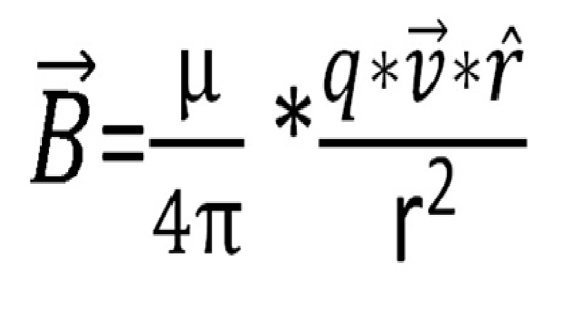
-In the above figure:  The relative Moon’s trace (not the Moons’ orbit) in 12 hrs is demonstrated (from Moonrise till Moon set) in 2D coordinates, the larger half of the circle (from A to B through under part) is not viewed. Within this duration, the Earth completes almost a half of cycle around its own axis. We can imagine that a certain observer standing somewhere near either North or South Pole, with a restricted view she/he can observes the Moon rising like depicted in the figure (while the Moon after Moonset is not seen, and the Earth makes no move).

The problem becomes pure geometric on 2D coordinates; and the figure requires some additional assumptions and quantities:

+Moon is at a general position (M) on sky, its distance to P is ‘’r’’ which varies against time and reaches the given value of d at meridian passing;

+Moon is rising at A and setting at B;

+Moon is expecting to pass meridian at Z over P; where angle APM=angle APZ =90⁰ while Moon’s altitude reaches its max of that day 75.7⁰.

+Vector  ''v'' is perpendicular to the radius that drawn through Moon (OM);

+PD is perpendicular to OM and parallel to;

+The angles are named after each point and numbered: M1, M2 and O1,O2; or P1,P2,P3,P4;

+Parameters: d=378521*10³m (minimum distance from the given position P to Moon’s centre).

+The Moon’s angle (P2 or angle APM) is taken by a professional equipment (Sextant) (at the given time); (the ‘’altitude’’ of Moon or any object on sky is understood as the angle between the line from observer to the object and horizontal plane at observer. Therefore, a large gap between the two aforementioned concepts (altitude and P2) is found, and no chance for a mixing up or confusion). Nonetheless, we can’t deny that the Moon’s altitude depends on P2 and reaches max almost at the middle of Moon’s trace between A and B, therefore we may keep considering altitude in relation with Moon’s angle P2. Furthermore, by the laws of 3D trigonometric, we can calculate P2 from altitude or vice versa, but no discussion for that issue is encouraged in this book.

The following is a figure that depicts approximately the altitude of Moon and the Moon’s angle P2:

 Figure 9/V-Moon’s altitude

(At Moon’s meridian passing, the angle APM is obviously 90⁰ or ½ π while Moon’s altitude keeps varying (angle MPH is not always to be 90⁰ even if we measure it from Earth equator)).

Again, we refer to the basic expression of Biot-Savart:

With Biot-Savart expression, this problem is the normal geometric one in astrophysics, we can demonstrate every important parameter on 2D coordinates. The sensitive issue in this expression is the product of vector ''v''  and unit vector ''r'', a vector directs from this page toward reader, and its  non-directional value is:

v*Sin(M1)

The non-directional value of B is:

b/1- To seek for (r ):

+Consider the triangle MDP (Vector ''v'' and PD are extended for a better view with M’P’//MP):

 Cos(O2)=Cos(07.95⁰)=0.990389

+In the triangle MPO:

In the triangle ODP:

OD=Re*Cos(O2)= 6356.8*0.990389=6295.704795 km

And Sin (M1) = Sin(81.91⁰+07.95⁰)=0.99999

MD = MO-OD or MD=(Re+d)-Re*Cos(O2)=6356.8+378521-6356.8*0.990389=

=378582.0952048 Km

Thus, r=MD/Sin(M1)= 378582.0952048/0.99999 =378585.88106 km=

r=378585.88106*10³m.

b/2-Angle M1:

M1=P2+P3 (Vector v is parallel with PD, the rule for alternate angles is applied)

P2 is Sextant reading (or astronomy almanac), and the P3=O2. Thus:

Angle M1=P2+O2, with given P2=81.91⁰ and P3=07.95⁰   

 Angle M1=81.91⁰+07.95⁰=89.86⁰ = 89051’’

Final calculation:

-Replace the followings in the expression and calculate value of B(tc):

Radius r=378585.881*10³m

Speed v=21230.8834 m/s

Angle M1=89⁰51”, Sin(M1)=0.99997≈1.

As assumption of this problem, q=Qm Coulomb, every length is in meter (m), the unit of B is Tesla (T).

We have:

B(tc)=10^-7*21230.8834*378585.881^-2*10^-6*Qm=

=1.481287*10^-20*Qm Tesla

(The previous approximate calculation gives result: B(tc)=1.439480*10^-20*Qm)

Because every of (r,v,M1) is depending on observer’s position, therefore the above result cannot be used for everywhere. Nonetheless it is to confirm that the Moon exerts its static electric force on the

Earth and especially induces a magnetic field on it, the value can be calculated.

For instant, a reading on a Tesla meter is indicating that the Moon’s contribution at Houston (South U.S.A) reaches its max +5*10^-7 T (normally the meter reading about 2-3 hrs before meridian passing can indicate the average magnetic level); we can find Moon’s total charge as following:

B(tc)= 1.481287*10^-20*Qm=5*10^-7 Tesla

Qm=B(tc)/ 1.481287*10^-20=5*10^-7/ 1.481287*10^-20 =

=3.375443*10¹³ Coulombs.

Everywhere inside the loop, the magnetic vector is by right-hand law.

(Problem: (the following problem is designated for 60 N to make sure that Moon signal is detected without being totally barred by plasma sphere): 3.375443*10¹³ Coulombs is a value of Moon’s charge that we detected when semi-moon (illumination 50%) is passing meridian of a position ‘’P’’ (60N, 0.0). If in 36 hrs later, when Moon’s illumination of 40% we detect Moon’s charge to be ‘’0’’ at a certain position P’ (60N, 180.0). Calculate the Moon’s total charge components Qa & Qb? 

This theoretic problem is definitely inspired by many science students but not included in this book. After this problem, we find out more about the roles of 2 hemispheres of Moon on E.M).

Figure 13/V-Earth’s magnetic field amplitude (in mG)

The above is a real graph of magnetic amplitude observed by our correspondent at latitude 70 N on Atlantic, about new moon. The records are bold for 10 minutes before and after the Moon’s meridian passing.