CHAPTER IV-MAGNETISM AT THE POLES

TWIN CONES AT POLES 

https://www.amazon.com/dp/1799165647

https://www.amazon.com/dp/B07PG44BMG

.

 

Figure 23/VI-Every Δ delta stacked on the others.

Figure 24/VI-Sun-Earth-Moon on sky

THIS BOOK CERTAINLY DOES NOT PRESENT EVERYTHING ABOUT EARTH MAGNETISM, AND THE AUTHOR BELIEVES THAT THERE ARE DEFINITELY STILL LOT OF PROBLEMS FOR EARTH MAGNETISM TO BE SOLVED.

CHAPTER III-MOON'S TOTAL CHARGE

MOON's TOTAL CHARGE ON E.M

Every previous solution is solved with many assumptions. Anyhow, the results are meaningful; they do confirm that the semi-moons in every day of Moon are approximately the reverting points when the Moon’s hemisphere effect changes from negative to positive or vice versa. Hence the two semi-moons divide the Moon’s orbit into 2 different, opposite halves; the effect on one half is going against or contrarian the current E.M, while the other’s effect is supporting or backing the current E.M.

The radiation from the Sun is changing and the Moon charge therefore is changing accordingly; so there must be a sequent change in Moon’s effect on E.M, and this chapter is a discussion about the change in circumstance when Moon’s charge is changing and the total charge ‘’Qa+Qb’’ is no more a ‘’0’’.

We leave the influence of permeability of the media between Moon and Earth centre for another problem; just consider the Moon’s influence on Earth’s surface.

Let’s set and solve the following problems for Moon’s effects.

2/-The problem of Moon’s total charge for Houston:

Houston of U.S chosen as observer in this problem is rather close to Earth's equator and quite in the middle of Van Allen belt and plasma sphere; therefore, it is very hard to detect the Moon’s effect. Nonetheless, we keep working with that location as observer then sort out the issue, and following is the problem:

U.S observer location (30N, 95W), USA on 02^nd May 2017, Moon’s total charge Qm and other parameters:

-Illumination: 49.1%≈50%, this is to make sure that each of the two hemispheres is capable to eliminate the other, so the hemispheric effect can be null.

-Meridian passing: 19.31 hrs.

-Moon rise/set (excerpt from Moon’s time table):

-Distance: 377652 km from point P to Moon.

-Moon’s average radius: R=1738.1 km.

Question:

With Moon’s total charge Qm≠0, consider the amplitude of magnetism that directly induced by Moon on Houston at 19.00 hrs LT.

2/1-To understand more about the question (analysis):

-The meridian passing is on 19.31 hrs at 75.7⁰.

-From the Moon’s timetable: Moon rise/set is 12.38/(next day)02.20 hrs. or 12.38/26.20  (or Moon’s on sky within 822 minutes).

-The distance from A or B to a general P (on longitude of P) can be viewed as the same and depicted in the following figure:

  

-The given P is on land surface with eye height ‘’0’’, the horizon viewed from P is a plane with the straight line from Sunrise (A) to Sunset (B).

-Note that AP = PB, by Pythagorean theory AP=(AO²-OP²)^1/2 (Figure 4/IV), where OP=Re, the value of Earth average radius despite ‘’O’’ is not coinciding on Oe (Figure 5/IV).

-A circle with centre (O) is designed to meet AP=(AO²-OP²)^1/2 and distance from P to Moon 377652 km. This centre (O) may not be coinciding on the terrestrial geometric centre (Oe).

 2/2-Solution:

2/2/1-Step 1: to re-think about the real things.

Like any other electric current or moving charge, the Moon definitely contributes magnetism. Moon’s total charge has been assumed as neutral with 2 opposite hemispheres in previous problem.

But in reality the total charge of any object under solar wind can’t be neutral at all the time; it is actually changing, and is given a value Qm (positive) in this problem.

The questions are how magnificent is the magnetism induced by the lunar total charge? Which wise (north or south) does it direct to?

2/2/2-Step 2: Assumptions.

- P (30N, 95W) is assumed as the stance for observer with eye height ‘’0’’.

- Distance from P to A is the same as P to B or any position on the longitude of P to those 2 positions of Moon.

-The Moon is assumed as on ‘’no real move’’ throughout the time of calculation. By this condition, the Moon’s real move is not considered. Instead, we consider the Moon’s relative move or 12(+) hr. trace around the Earth.

-Moon’s total charge (Qm=Qa+Qb and Qm≠0) stays unchanged throughout this calculation.

-Distance: 377652 km is from P to the nearest position of the Moon. The distance from P to charge centre of Moon can be approximately added with ½ of Moon’s average radius 1/2*1738.1 km.

The distance d=378521 km is assumed as distance from observer to Moon’s charge centre.

3-Step 3: Solution with reliable accuracy.

-Recall Biot-Savart expression for a single charge. We add some more lines on the basic figure 12b/v to facilitate the solution.

-In the above figure:  The relative Moon’s trace (not the Moons’ orbit) in 12 hrs is demonstrated (from Moonrise till Moon set) in 2D coordinates, the larger half of the circle (from A to B through under part) is not viewed. Within this duration, the Earth completes almost a half of cycle around its own axis. We can imagine that a certain observer standing somewhere near either North or South Pole, with a restricted view she/he can observes the Moon rising like depicted in the figure (while the Moon after Moonset is not seen, and the Earth makes no move).

The problem becomes pure geometric on 2D coordinates; and the figure requires some additional assumptions and quantities:

+Moon is at a general position (M) on sky, its distance to P is ‘’r’’ which varies against time and reaches the given value of d at meridian passing;

+Moon is rising at A and setting at B;

+Moon is expecting to pass meridian at Z over P; where angle APM=angle APZ =90⁰ while Moon’s altitude reaches its max of that day 75.7⁰.

+Vector  ''v'' is perpendicular to the radius that drawn through Moon (OM);

+PD is perpendicular to OM and parallel to;

+The angles are named after each point and numbered: M1, M2 and O1,O2; or P1,P2,P3,P4;

+Parameters: d=378521*10³m (minimum distance from the given position P to Moon’s centre).

+The Moon’s angle (P2 or angle APM) is taken by a professional equipment (Sextant) (at the given time); (the ‘’altitude’’ of Moon or any object on sky is understood as the angle between the line from observer to the object and horizontal plane at observer. Therefore, a large gap between the two aforementioned concepts (altitude and P2) is found, and no chance for a mixing up or confusion). Nonetheless, we can’t deny that the Moon’s altitude depends on P2 and reaches max almost at the middle of Moon’s trace between A and B, therefore we may keep considering altitude in relation with Moon’s angle P2. Furthermore, by the laws of 3D trigonometric, we can calculate P2 from altitude or vice versa, but no discussion for that issue is encouraged in this book.

The following is a figure that depicts approximately the altitude of Moon and the Moon’s angle P2:

 Figure 9/V-Moon’s altitude

(At Moon’s meridian passing, the angle APM is obviously 90⁰ or ½ π while Moon’s altitude keeps varying (angle MPH is not always to be 90⁰ even if we measure it from Earth equator)).

Again, we refer to the basic expression of Biot-Savart:

With Biot-Savart expression, this problem is the normal geometric one in astrophysics, we can demonstrate every important parameter on 2D coordinates. The sensitive issue in this expression is the product of vector ''v''  and unit vector ''r'', a vector directs from this page toward reader, and its  non-directional value is:

v*Sin(M1)

The non-directional value of B is:

b/1- To seek for (r ):

+Consider the triangle MDP (Vector ''v'' and PD are extended for a better view with M’P’//MP):

 Cos(O2)=Cos(07.95⁰)=0.990389

+In the triangle MPO:

In the triangle ODP:

OD=Re*Cos(O2)= 6356.8*0.990389=6295.704795 km

And Sin (M1) = Sin(81.91⁰+07.95⁰)=0.99999

MD = MO-OD or MD=(Re+d)-Re*Cos(O2)=6356.8+378521-6356.8*0.990389=

=378582.0952048 Km

Thus, r=MD/Sin(M1)= 378582.0952048/0.99999 =378585.88106 km=

r=378585.88106*10³m.

b/2-Angle M1:

M1=P2+P3 (Vector v is parallel with PD, the rule for alternate angles is applied)

P2 is Sextant reading (or astronomy almanac), and the P3=O2. Thus:

Angle M1=P2+O2, with given P2=81.91⁰ and P3=07.95⁰   

 Angle M1=81.91⁰+07.95⁰=89.86⁰ = 89051’’

Final calculation:

-Replace the followings in the expression and calculate value of B(tc):

Radius r=378585.881*10³m

Speed v=21230.8834 m/s

Angle M1=89⁰51”, Sin(M1)=0.99997≈1.

As assumption of this problem, q=Qm Coulomb, every length is in meter (m), the unit of B is Tesla (T).

We have:

B(tc)=10^-7*21230.8834*378585.881^-2*10^-6*Qm=

=1.481287*10^-20*Qm Tesla

(The previous approximate calculation gives result: B(tc)=1.439480*10^-20*Qm)

Because every of (r,v,M1) is depending on observer’s position, therefore the above result cannot be used for everywhere. Nonetheless it is to confirm that the Moon exerts its static electric force on the

Earth and especially induces a magnetic field on it, the value can be calculated.

For instant, a reading on a Tesla meter is indicating that the Moon’s contribution at Houston (South U.S.A) reaches its max +5*10^-7 T (normally the meter reading about 2-3 hrs before meridian passing can indicate the average magnetic level); we can find Moon’s total charge as following:

B(tc)= 1.481287*10^-20*Qm=5*10^-7 Tesla

Qm=B(tc)/ 1.481287*10^-20=5*10^-7/ 1.481287*10^-20 =

=3.375443*10¹³ Coulombs.

Everywhere inside the loop, the magnetic vector is by right-hand law.

(Problem: (the following problem is designated for 60 N to make sure that Moon signal is detected without being totally barred by plasma sphere): 3.375443*10¹³ Coulombs is a value of Moon’s charge that we detected when semi-moon (illumination 50%) is passing meridian of a position ‘’P’’ (60N, 0.0). If in 36 hrs later, when Moon’s illumination of 40% we detect Moon’s charge to be ‘’0’’ at a certain position P’ (60N, 180.0). Calculate the Moon’s total charge components Qa & Qb? 

This theoretic problem is definitely inspired by many science students but not included in this book. After this problem, we find out more about the roles of 2 hemispheres of Moon on E.M).

Figure 13/V-Earth’s magnetic field amplitude (in mG)

The above is a real graph of magnetic amplitude observed by our correspondent at latitude 70 N on Atlantic, about new moon. The records are bold for 10 minutes before and after the Moon’s meridian passing.

CHAPTER II/p2-TWO OPPOSITE HEMISPHERES OF MOON

TWO OPPOSITE H.S OF MOON

Moon is the only satellite to Earth. In human life, the Moon merges in poet, music and children’s daily dream.

Since 50^th of last century, human being had succeeded in researching the Moon, U.S scientists even launched in there and planned to build an outpost on it, their plan is still going on.  Nonetheless we don’t discuss about their plan, but we do discuss about another issue: the charges on Moon and their influence to the Earth.

We denote magnetic compositions contributed by Moon’s hemisphere the Δ4, Δ5 and Δ6 where Δ4 is for negative hemi-sphere influence, Δ5 is for positive hemi sphere; and Δ6 is for total charge contribution.

The following is charged Moon that depicted by NASA:

The ion wind from Sun is striking on Moon’s surface and energizing the electrons on there, as NASA’s argument, the direct result is to electrify the shined part positively. The highly energized electrons flock to settle on the dark side of the Moon where they lost their energy. That’s how the Moon surface is such illustrated in the Image 1/v. In order to clarify the Moon’s hemisphere effects on Earth, we set and solve the following problem.

1-Problem 1: The lunar hemisphere effect.

Under sunlight, the Moon is a charged or an electrified object. Suppose that the nature of object is neutral and so the positive charge on shined side is balanced against the negative charge on the dark side.

Conclusion for solution 1:

The opposite hemi-spheres of Moon induce magnetism on P(Houston). As seen in the figure 6/v above, Qb is nearer to Earth; by the inverse law of electric force, Qb can influence more than Qa.

Moon is considered as stationary during the Earth is rotating, so Moon’s magnetic vector is parallel with Earth’s rotation axis and consists of X and D compositions.

Qb might be negative which induces a contribution that heads to North, against current Earth’s magnetism.

The result of calculation (6.241*10^-23*Qb Tesla) is not too tiny because Qb is still unknown and varying at all the time. If we give Qb or Qa a certain figure such as 10 6 Coulombs, we may have B(hs), but we don’t do it now as our discussion is still going on.  

CHAPTER I/p2-VAN ALLEN BELT CONTRIBUTION

VAN ALLEN BELT

I-General about Van Allen belts:

I and many among my colleagues used to view Earth’s magnetic field as one that can only facilitate the magnetic compass to indicate the North magnetic direction and no more it can offer. But the Van Allen belt appears to change our mind; the Earth’s magnetic field is not very strong but good enough in facilitating the establishment of Van Allen belt which can stop any fast moving charged particle. The Van Allen belt, as matter of fact, plays an important role in protecting our planet.

(The following is almost prepared with close reference to SPACE & NASA’s documents and papers, which are open to everyone and nothing is from classified information.)

(By NASA)

1-What is Van Allen belt: a collection of charged particles, gathered by Earth’s magnetism, in a shape of belts around Earth.

2-The earliest discovery to the belts: 1958 by Explorer 1 (NASA’s Satellite).

-Belt’s structure: normally 2 belts, one is separated from the other by a large drain/gap; can split up to 3 belts or merged in one sometimes. The inner belt is almost close to Earth surface at minimum about 400 miles; while the outer belt is rather far and even stretches to 36000 miles.

The drain is discovered in 2012; a remarkable feature of the belt is that its drain can stop the ultra-fast electron in there. The scientists from NASA are still not determined about reason for the belt separation. Their hesitation is quite understandable because no mechanism of electric force or magnetic field is found linking to the wax & wane activity of the belts (which is in conjunction with Sun’s activity). The scientists likely ascribe to the particles from space or the Sun.

The unidentified particles or quarks might be gathered among the belts and create an unknown field between them, the field makes the belts split-up wide.

-How the belts work: They can wax and wane in response to incoming energy from the Sun, sometime swelling up enough to expose satellites in low-Earth orbit to damaging radiation.

-Undiscovered about the belts: With some satellites working on space at all the time; the more research to the belts are carried out, the more expect to be discovered; even the unidentified particle or quark.

-Plasmasphere: A companion to the belts is a giant plasma sphere which can be assumed as twinned to the belts. The plasma sphere is cloud of relative cool and charged particles that fills the outermost region of Earth’s atmosphere. That sphere begins approximately at 400-600 miles (rather close to Earth surface) and extends partially to outer Van Allen belt.

PROBLEM

If total charge of the Van Allen belts and plasma sphere is equivalent to a single band of +10⁶ Coulombs around Earth equator at a distance 1500 km from Earth surface, and evenly distributed on it.

How is the magnetism induced by the Band to the equator (Earth)? 

(V-A 01)

   

    

Where unit of ‘’Q’’ is in Coulomb and unit of ‘’d’’ is km.

Replace Q=10⁶ Coulombs, d=1500 km (as assumed) into the above formula:

  Δ(3)= -8.4169*10^-23 *666.666667=10^-20*5.611267 Tesla

(Note: the Belt is assumed as on a plane perpendicular to Earth’s rotating axis, the assumption is not verified and the reality definitely is not be so. Therefore, in order to calculate for a better accuracy, the belt as well as the plasma sphere can be represented by many bands (or hoops) in a larger problem).

Conclusion:

If Van Allen belt and plasma sphere are equivalent to a band of Q Coulombs (the Band) around the Earth on plane of Earth’s equator. The Band is to induce magnetism on Earth’s equator; its additional intensity is calculated as (V-A 01):

 

In reality, Van Allen belts and plasma sphere are not only changing in shape and size, but also in intensity. With such a complicated change, the above mentioned ‘’Δ3’’ demonstrates nothing but ‘’yes’’ to the question ‘’influence?’’. Furthermore, as noted above, the larger problem is required to estimate the additional magnetic intensity with better accuracy.

PART II

EXTERNALITIES OR ASTRONOMY ON E.M

CHAPTER II/p1-SEA VS LAND

PROBLEMS OF SEA vs LAND CHARGEs

The last chapter presented a discussion about positively charged land surface and the negatively charged sea surface. They both are parts that constituted the Earth and moving together with Earth’s rotation; if the charge of each is opposite to the other, then each induces magnetism that contrarian to the other. In the paragraph 2 (Argument of electric paradox) we even discussed and mentioned the average ratio +ions/-ions in every CC of air on land.

However, we leave that ion ratio for another discussion and work with graph of thunderstorm coverage for our problem in this chapter. So we set and solve the following problems with an assumption that: total contribution of every charged cloud on the Earth is ‘’nil’’ throughout our problem solution.

I-PROBLEM OF A SINGLE CHARGE ON THE EARTH SURFACE:

1-Problem:

-A charge of -100 Coulombs, locating at a fixed position P (30N, 100E) on surface a globe model of 100 m radius. Another charge +100 Coulombs, locating at the same fixed P on altitude h=10 m above surface of globe. How is magnetism induced by those 2 charges to rotation axis if its rotation is the same as Earth’s cycle (24 hrs)?

a-Analyse:

This figure is displaying a global coordinate, where ‘’O’’ is centre and P is a given point on global surface.

The latitude of P is also the angle ‘’ϕ’’ between OP and equator’s plane.

Figure 1/II-Charge at P versus P1 on global coordinates (not in scale).

The imaginary plane whereby the P moving on is the plane of latitude slice at 30N- depicted in the next figure.

The distance from P to global rotation axis is the value of ‘’r’’ in our calculation:

PP2=r=R*cos(ϕ)

The distance from P1 to global rotation axis is another value of ‘’r₁’’ in our calculation:

P1P1’=r₁=(R+10)*cos(ϕ).

The global rotation is to carry P and P1 together. In scope of electromagnetism, longitude of P (100 E) plays no role or helpless in our calculation.

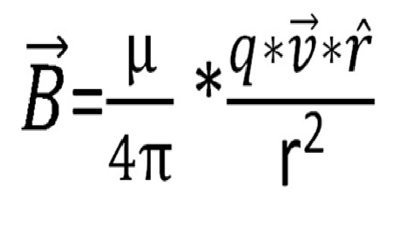
The globe is rotating around its own axis at all the time. The ‘’P’’ is fixed on globe’s surface and moving along with global rotation. Every single charge moving around a certain point is to create a loop of electric current by which the magnetism is induced. The following is Biot-Savart expression (9.1.20) to facilitate our calculation:

B=(μ/4π) * (qv*''r''/r(2))

(v is speed vector of a charge and ''r'' is unit vector of radius, the vector is not presented properly in this blog)

========Note

Permeability (μ) of the medium material between both P,P1 and globe rotation axis: As we are working with Earth model, therefore we suppose its permeability to be one of Earth, the average of Iron (99.95%) (Because Earth core is assumed as Iron), and normal air (µ0 =4π*10-7 N/A2). In reality µ is varying, the permeability at different place is different. This is only to set a way to solve the real problem. ==========

b-Assumptions: In order to solve this problem, we need some assumptions.

-The globe’s average radius R=100 m so:

 r=R*cos(ϕ)=100*cos(30⁰)=86.6 m

r₁=110*cos(30⁰)=95.26 m

-Permeability of the medium material between P,P1 and globe rotation axis: As we are working with Earth model, therefore we suppose the permeability as one of Earth, the average of Iron (99.95%) (Because Earth core is assumed as Iron), and normal air (µ₀ =4π*10^-7 N/A²). So we have: 

µ=1/2 (0.25+4π*10^-7) =0.12500126 N/A²

General formula for speed (v) of P: v=2πr/24*60*60 m/s, replace ‘’v’’ to Biot-Savart expression:

dB= *q/(r*48*60*60)=

dB=7.233869*10^-7*q/r (named as I-Biot-Savart).

Although the coefficient 7.233869*10^-7 is derived from µ, π and cycle (24 hrs), it is interpolated from Biot-Savart expression, so we name it as ‘’ interpolated Biot-Savart’’ or I-Biot-Savart for further reference.  

With I-Biot-Savart, the only dependent to location of the charge ‘’q’’ on the Earth is its distance to Earth’s rotation axis ‘’r’’, while ‘’q’’ is to be found out.

Thus, we can be proud to say: if I have a charge and its location on the Earth, we find out how much it contributes to Earth Magnetism.

c-Solution with Biot-Savart:

Solution 1:

-Given charge at P: q=-100 Coulombs

-Radius of the loop: r= 86.6 m   

-Product of vector speed ‘’v’’ and unit vector ‘’r’’ is a vector that parallel with Earth’s rotation axis, pointing to true North and valued |v|, because vector  is perpendicular to unit vector .

-Value of Δb1 is calculated step by step with the above Biot-Savart interpolated as: =7.233869*10^-7*q/r=-7.233869*10^-7*100/86.6=-8.353197*10^-7

Solution 2:

-Given charge at P1: q1=+100 Coulombs

-Loop radius: 95.26m

-Value of Δb2 is also calculated step by step with the above Biot-Savart interpolated as:

=7.233869*10^-7*q/r1=7.233869*10^-7*100/95.26=

=7.593816*10^-7

d-Summary words: (apply I-Biot-Savart).

-8.353197*10^-7 + 7.593816*10^-7=

=-0.7593816*10^-7 Tesla

If two oppositely charged points of the same true value are placed on the same position at 2 different altitudes; resulting the distance from each to the rotation axis to be different to the other and the intensity of magnetism contributed by each charge is different to the other. The closer to axis, the more it contributes; that’s rule. The total of the two is in favour of the inner charge.

II-PROBLEM OF OCEANS VS CONTINENTS

1-Basic argument:

The Sun is rather far from Earth, so it can’t apply any magnetic influence on the Earth directly but indirectly through brokerage of atmosphere, continent and ocean surfaces. Beyond the influence that almost considered in the last chapters, this is a problem for the contributions of continent and ocean (or sea & land as I name them in this book) to the Earth Magnetism in the light of Biot-Savart laws.

2-Thunderstorm matter:

From atmospheric research, the thunderstorm area varies against the time with 24-hr revolution or daily cycle. The following is a graph that re-built by the data taken at Mauna Loa Observatory (Hawaii Islands):

Figure 3/II-This is observation result from Mauna Loa.

The graph is indicating that the Americas continent is the place of thunderstorm and lightning, while the less thunderstorm continent is Asia. The average thunderstorm continent is Africa which is at the same peak as Americas.  

The above figure is divided approximately into 3 trapezia and 1 rectangle to calculate the total area of thunderstorm and its average within 24 hrs. The result is the average area under daily thunderstorm ‘’80*10⁴ km²‘’, used as entry for our problem.

Figure 4/II-Global average area under thunderstorm daily.

Thunderstorm and lightning on 30 March 2017 (as instant only, the situation is changing at all the time).

Picture 5/II-An instant image (courtesy from Blitzortung.org)

The world thunderstorm map is indicating that the thunderstorm is covering almost within 55N to 55S, where some spotted lands should be mentioned in the South semi-sphere such as Australia, Indonesia. So, we consider a reasonable way to distribute the area of 80*10⁴ km² under daily thunderstorm, make those figures the entries to our problem.

Note: (Under the thunderstorm, the area is almost positively charged and assumed to be so).

Figure 6/II-Illustrative structure of a thunderstorm cell

(The above figure is re-built after many real flights through a super cell, the pilots who performed the flight surveys were recognised as braves in atmosphere research.

The obvious sign illustrated above is the positive land surface that expands as large as the thunderstorm cell is. The positive patch on land, as matter of fact, must be laid there until all the charges above to be discharged. Furthermore, the land surface is moving during Earth rotating with as high speed as V*cos(ϕ) (V-speed of any position at equator-463 m/s, (ϕ) is position’s latitude).

3-Problem:

Daily global average area under thunderstorm is 80*10⁴ km². If the land under thunderstorm is positively charged (supposed average +1000 Coulombs/km²); reciprocally the oceans are negatively charged so that they can balance with the land positive charge (P65-Bal.).

Assume that the land average height is 10 m above mean sea level, while sea level is assumed as at its average level during our calculation.

What is the contribution of sea and land to Earth’s Magnetism?

X

X                             X

There are obviously several ways to solve the problem. Our way is to attribute a certain charge to each potential location, calculate contribution of each and tantalize at the end of this section.

The seas (and oceans) are considered as one single electrode because salt water in ocean is homogeneous with high electric conductivity. The assumed value of electric charge is distributed evenly to everywhere of seas and oceans. We will calculate the ocean contribution to earth’s magnetism and summed up with contribution from lands.

3a-Solution-Land contribution (Δ1):

Expression I-Biot-Savart (p84) for Δ(i):  

Δ(i)=7.233869*10^-7*q(i)/r(i)

Back to our problem, it should be simplified by distributing approximately the total given land charge to 6 different places; each of them represents a specific locale where the thunderstorm land is dominating its region.

The land charge is estimated on basis of daily air-earth record (figure 4/II), and every charge is positive, furthermore as noted before that each diminishes the E.M.

From entry, we have 80*10⁴ km² area and assumed 10³ Coulombs/km²; so total charge on land is assumed as 8*10⁸ Coulombs. From every position, we always find the distance to Earth rotation axis (assume that average height of land charge is 10 m above average sea water level).

With approximately estimated percentage of areas under thunderstorm, we also attribute average area under thunderstorm for each different location. Eventually an assumed charge at each location can be found. A table of mock calculation is established as following:

-Assumption1: by percentage, the areas under thunderstorm with respective charges are approximately divided as following:

+America continental (AC): 20 pcts, (35N, 90W.)

With r(1)+10=5,207,195.7m, and q(1)=16*10⁷

+North Africa & Europe (A&E): 20 pcts, (40N, 20E.)

With r(2)+10=4,869,601.3m, and q(2)=16*10⁷

+South Africa (S.A): 10 pcts, (10S, 30E.)

With r(3)+10=6,260,235.9m, and q(3)= 08*10⁷

+Japan and its’ neighbour (Jap.): 15 pcts., (35N, 140E.)

With r(4)+10=5,207,195.7m, and q(4)= 12*10⁷

+Philippine and Indonesia (P&I): 15 pcts., (0.0, 115 E.)

With r(5)+10=6,356,810.0, and q(5)= 12*10⁷

+Australia (Aus.): 20 pcts. (25 S, 140 E.)

With r(6)= 5,761,227.3 m,  and q(6)= 16*10⁷

(Thunder cloud (negative) makes its opposite patch on land positive (see the super thunderstorm cell), each lightning discharges a lot of charge on both cloud and land charged patch. This is assumed as one of motivation to the surge of E.M every day. Therefore we think about the following problem.)

Figure 6b/II-Land charge (+) contribution-Δ(1)

As matter of fact, the contribution of a positive charge on Earth is contrary to current Earth Magnetism of the Earth.

Problem 1:

A thunder cloud patch of following properties:

-Coverage: 10 km²

-Average negative cloud height: 2000 m

-Location: 30N, 90W as coverage’s centre.

-Total charge: 10⁶ Coulombs.

There is no more charge on cloud left, or the total 10⁶ Coulombs will disappear after the lightning.

Question 1: if we consider the contribution of thunder cloud to E.M, what are the contributions of both cloud and its opposite patch on land to E.M?

Question 2: How is the surge in E.M caused by the lightning?)

This problem is not solved or discussed in this book.

3b-Solution-Ocean contributions (Δ2): We call back I-Biot-Savart.

Δ(i)=7.233869*10^-7*q(i)/r(i)

From ocean facts, the four oceans are covering 70% of global area. Every ocean is connected to the others, the water in ocean is salted and always at high electric conductivity; therefore sea water is considered as homogeneous as a single electrode in relation to any other object.

As assumption in the entry of this problem, our globe is assumed as a neutral object, so the total electric charge is ‘’nil’’. Because the land is charged as counter part of thunder cloud, so the oceans must have charge that opposite to land for neutralizing the land charges. By this argument, we consider the total sea-charge equal to total land-charge and evenly distributed on every ocean and seas connected to them.

Figure 7/II-Globe with Longitude-Latitude network

+From the air-earth current research, our calculation gives an approximate result for total land charge under thunderstorm +80*10⁴*1000 Coulombs. Therefore: 

Total Sea Surface Charge (SSC stands for them from now onward) should be as much as

-80*10⁴*1000 Coulombs or:

=-8*10⁸ Coulombs

We assumed that the total is maintained and distributed evenly over every ocean throughout our calculation.

+From the figure 7/II above, we divide the globe into 6 global chunks (horizontal bands from North down to South). Each chunk expands 30⁰ latitude, we calculate ‘’r’’ (distance to Earth’s rotation axis) from average latitude of the band such as 15 is average of 0-30; 45 is average of 30-60; 75 is average of 60-90.

 After the distance ‘’r’’ calculation, each band can be considered as a rim or a hoop by which the negative charge locates on. The figures are approximately assumed as following:

3/2/1-From 60N to North Pole including Artic, 20*10⁶ km²

Figure 8/II-Arctic and its substitute

-Distance to axis r(1)=Re*cos(75)=1,645,216 m

-Water surface area: 19,889,355 km²

Figure 9/II-Band of 30N-60N latitude degrees and its substitute.

-Distance r(2)=Re*Cos(45)=4,494,936.4 m

-Water surface area: 44,745,958 km²

Figure 10/II- Band of 0-30N latitude degrees and its substitute

Distance to rotation axis: r(3)=Re*Cos(15)=6,140,197 m

Water surface area: 74,576,252 km²

Figure 11/II-Band of 0-30S latitude degrees and its substitute

Distance to rotation axis: r(4)=r(3)=Re*Cos(15)=6,140,197 m

Water surface area: 119,322,568 km2

Figure 12/II- Band of 30-60S latitude degrees and its substitute

Distance to rotation axis: r(5)=r(2)Re*Cos(45)= 4,494,936.4 m

Water surface area: 80,542,806 km2

Figure 13/II- Antarctic and its substitute

-Distance to axis r(6)=r(1)=Re*cos(75)=1,645,216 m

-Water surface area:  14,915,671 km²

X

X                                             X

We are dividing the globe into 6 chunks or bands, each is far from Earth’s rotation axis at an average distance, denoted as r(i) where ‘’i’’ is varying from 1 to 6. We also attribute approximately a certain sea surface area to each chunk in condition that total charge can balance +8*10⁸ Coulombs of all continent summed up.

We have calculated Δ(1) the land contribution to E.M, now we do the same to find out sea surface contribution Δ(2) to E.M. Our job at this stage is to figure out how the 6 chunks contribute to E.M.

Solution:

Total area: 352,876,000 km2,

Charge per s.km: -8*10⁸/352,876,000=-2.267085 Coulombs/km²

We have every q(i) for respective chunk as following:

q(1)= -2.267085*19,889,355=-45,090,858 Coulombs

q(2)= -2.267085*44,745,958=-101,442,890 Coulombs

q(3)= -2.267085*74,576,252=-169,070,702 Coulombs

q(4)= -2.267085*119,322,568=-270,514,404 Coulombs

q(5)= -2.267085*80,542,806=-182,597,387 Coulombs

q(6)= -2.267085*14,915,671=-33,815,094  Coulombs

We again do apply I-Biot-Savart or Biot-Savart 9.1.20 to each chunk from North to South:

Δ(i)=7.233869*10^-7*q(i)/r(i):

-With r(1)=1,645,216 m, q(1)=-45,090,858 Coulombs

 Δ(w1)=-1.982605*10^-5

-With r(2)=4,494,936 m , q(2)=-101,442,890 Coulombs

Δ(w2)=-1.632558*10^-5

-With r(3)=6,140,197 m , q(3)=-169,070,702 Coulombs

Δ(w3)=-1.99185*10^-5 

-With r(4)= 6,140,197 m, q(4) =-270,514,404 Coulombs

Δ(w4)=-3.1869755*10^-5 

-With r(5)=4,494,936 m, q(5)= =-182,597,387 Coulombs 

Δ(w5)=-2.938608*10^-5 

-With r(6)=1,645,216 m, q(6)= =-33,815,094 Coulombs

 Δ(w6)=-1.48682*10^-5    

10.56539*10^-5 Tesla is equivalent to a magnetic composition induced by a charge of 9,315,354.9532*10⁷ Coulomb at Earth equator.

And -13.219416*10^-5 Tesla is equivalent to a magnetic composition induced by a charge of -11,655,372.145666*10⁷ Coulombs at Earth equator.

Figure 14/II-Sea Surface contribution to E.M

Contribution from a negative charge on the Earth is always co-adapted with present Earth Magnetism.

4-Auto-offset Mechanism of the Earth Magnetism:

The aforementioned problems point out that the more positive charge on Earth surface, the more power is taken away from Earth Magnetism. Meantime, for the same speed of a charge crossing perpendicular at the field lines of Earth Magnetism; the more powerful Earth Magnetism, the more powerful force from Earth Magnetism applies on the charge.

Figure 14a/II-Opposite magnetic forces on opposite charged ions

The above mentioned mechanisms lead to a speculation: with the magnetic forces applied on the free ions in the clouds on sky, the Earth Magnetism can offset its magnitude.

That speculation needs to be verified with more test and considerations.

CONCLUSIONS (for part I):

-In addition to underground rotors, the land charges (figure 6b/II) and sea surface charge (SSC), (figure 14/II) contribute to the E.M. Although the land charges as well as sea surface charge are belonging to the Earth but totally influenced by external variableness regardless how we denote it.

-Although those two problems are set and solved with assumed figures, the results are demonstrating that:

+The total of Δ(1)+Δ(2) is on favour of Δ(2), indicating that the influence of the sea is more than that of the land, and supporting E.M or adding on it.

Figure 14b/II-The equivalent of sea&land charges/24 hrs.

+The lightning producing jolt: lightning frees the charges for both thunder cloud and its opposite patch on land; so as consequence of lightning, the Δ(1) must drop right away and considerably. The drop of Δ1 produces a huge magnetic jolt (total Δ(1)+Δ(2) soars due to Δ(1) drop) or the magnetic surge, demonstrated in daily E.M record. Although the lightning is viewed as motivation of every jolt or jerk in Earth Magnetism, but due to the retardation as well as the contribution of many other magnetic inducers, we can point out no direct involvement of lightning in any Earth Magnetism record.

-The divided Earth: might be divided by many different ways, the sum of Δ(1)+Δ(2) might be changed because of such different dividing; but the ultimate demonstration is unchanged and that: The negative charge on sea surface stands up to the positive charge on land surface on term of influence to E.M.

-The solutions to those above problems are leading to a direct relation between Sun position and E.M intensity and E.M 24-hr cycle, but many other influences are piled on E.M and making 24-hr cycle faded. Nonetheless, such cycle will be in another discussion at the end of this book with Maxwell Equation. 

The last chapter presented a discussion about positively charged land surface and the negatively charged sea surface. They both are parts that constituted the Earth and moving together with Earth’s rotation; if the charge of each is opposite to the other, then each induces magnetism that contrarian to the other. In the paragraph 2 (Argument of electric paradox) we even discussed and mentioned the average ratio +ions/-ions in every CC of air on land.

However, we leave that ion ratio for another discussion and work with graph of thunderstorm coverage for our problem in this chapter. So we set and solve the following problems.